Home > Introduction > Tutorial > CALM Buoy Modeling

CALM buoy modeling tutorial

Introduction

The objective of this tutorial is to provide a practical example of how to model a typical CALM buoy, with a focus on coupled analysis in both the frequency domain (FD) and time domain (TD).

The tutorial emphasizes the buoy in its idle state (i.e., without a connected tanker), incorporating potential flow and Morison elements, as well as specific viscous drag damping for the buoy’s skirt and body. It also explores the coupling with mooring lines and Oil Offloading Lines (OOLs), and includes both static and modal analysis. Finally, the session defines a set of dynamic analyses to be performed in either the frequency or time domain.

Table of Contents

1 Global Model Description
    1.1 Buoy Mooring Lines
    1.2 Offloading Lines
    1.3 Model Excel Datasheet
    1.4 Coupled Anaysis
2 STEP 1: Define a Generic Floater and import a Mesh
    2.1 Define a preliminary floater motion type
    2.2 Launch 1st order diffraction/radiation and Generate the HDB file rev01
    2.3 Tips for Symmetrical Mesh
    2.4 End of Step 1 and Resulting HDB file rev01
3 STEP 2 : Complete Model Definition
    3.1 Floater motion update
    3.2 Buoy own Mass and Inertia terms
    3.3 Buoy viscous damping
    3.4 Buoy mooring lines and fairleads
    3.5 Buoy mooring lines
    3.6 Lines definition
    3.7 Offloading system
    3.8 OOL internal fluids
    3.9 TurnTable and Hawser Setup
    3.10 Ballast definition
    3.11 Static check
    3.12 Definition of a Frequency Domain and checks
4 STEP 3 & 4 : Update of HDB file with motions RAOs
    4.1 Select the FD analysis for the RAOs motions computation and update the HDB file (with or without 2nd order loads)
    4.2 Update the floater motion type
5 STEP 5 : Example of fatigue DLC
    5.1 Fatigue Analysis - Input Data
        5.1.1 Wave Energy Distribution – Direction 25°
        5.1.2 Wave Energy Distribution – Direction 35°
    5.2 Wave Energy Distribution – Direction 50°
    5.3 Fatigue analysis : DLC definition
    5.4 Fatigue Analysis : DLC runs

Global Model Description

The model is composed of :

• Offloading lines

• CALM buoy moored by 3 clusters of 3 lines

• FPSO

In this tutorial, focus is put on the CALM buoy (FPSO is a fixed point). The water depth is 752m.

Parameters	X (m)	Y (m)	Z (m)
Buoy ref point in Global frame	0	0	0
FPSO ref point in Global frame	-2000	0	0
OOLs oriented along X global axis

Table 1 : Geometric positions.

Parameters	Value	Unit
Buoy Body	23	m
Buoy well diameter	6.2	m
Buoy Body height	10	m
Skirt Diameter	27.58	m
Top of skirt from keel	1	m
Skirt WT	0.18	m
ChainStopper from keel	0.82	m
Buoy body Mass	1004.5	t
COG Position/center	0	m
Cog Vertical Position/keel	6.17	m
Operational Draft	6	m
Ixx roll inertia in air @COG	49778	tm²
Iyy pitch inertia in air @COG	49778	tm²
Izz yaw inertia in air @COG	66411	tm²

Table 2 : CALM buoy parameters.

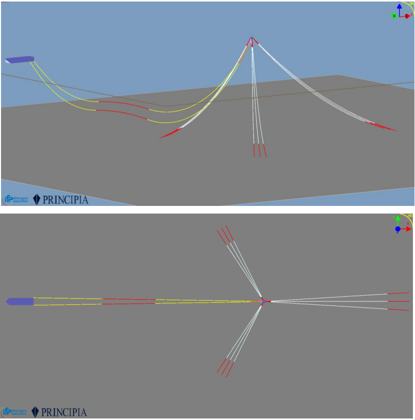
Figure 1 : view of whole system model.

Buoy Mooring Lines

The following tables present the lines geometrical paremeters and composition for mooring lines. Buoy fairleads are 0.82m above keel.

Composition	Top Chain	Wire	Bottom Chain	Total	Unit
Front lines	62	813	160	1035	m
Back lines	62	1159	190	1412	m

Table 3 : Offloading lines geometrical parameters.

Mooring Lines Azimuths	-	-	-	Unit
Legs 1, 2, 3	236.5	240	243.5	deg
Legs 4, 5, 6	-3.5	0	3.5	deg
Legs 7, 8, 9	116.5	120	123.5	deg

Table 4 : Mooring lines azimuths.

Element	Value
Top chain	Chain_125mm
Wire	Cable_58mm
Bottom chain	Chain_125mm

Table 5 : Mooring lines composition.

Element	Value	Unit
Buoy radius	12.65	m
Long legs - Anchor radius	1200	m
Short legs - Anchor radius	700	m

Table 6 : Buoy radius and mooring radius.

Element	Value	Unit
Short Legs pretension	77	tons
Long Legs pretension	153	tons

Table 7 : Mooring lines pretensions.

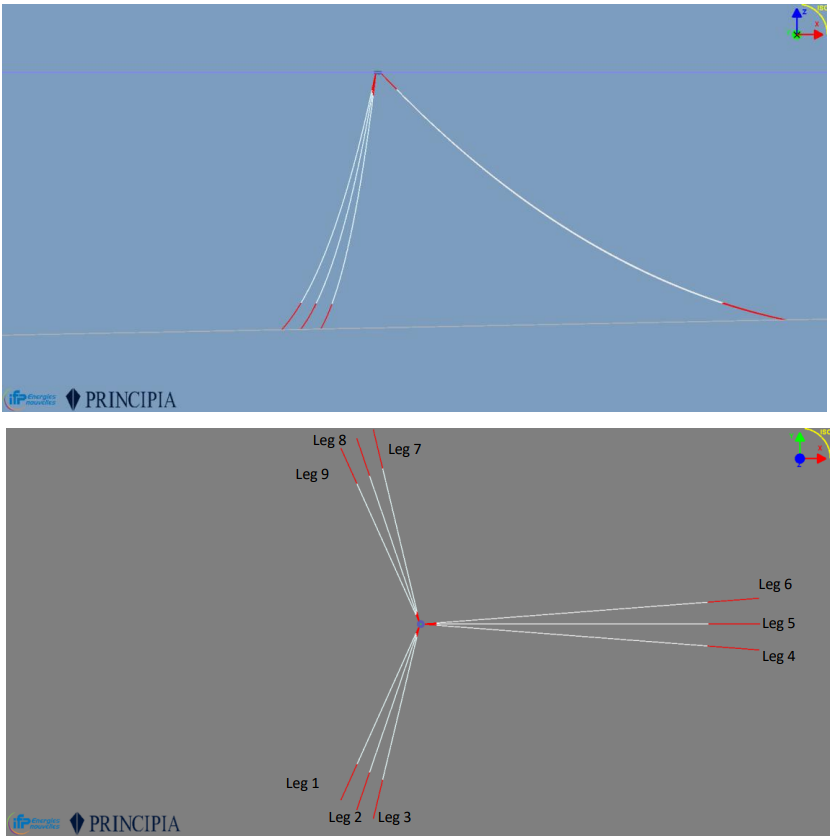
Figure 2 : Legs numerotation.

Oil Offloading Lines (OOLs)

OOL configuration	UPPER	LOWER	m
Standard_FPSO	675	725	m
BM	450	450	m
Standard_Buoy	875	925	m
Reinf1	146	146	m
Reinf2 Buoy_side	54	54	m
Total	2200	2300	m

Steel OOL	Value	Unit
OD (20")	508	mm
WT nominal	22.2	mm
WT reinf1	25.4	mm
WT reinf2	30	mm
Steel Grade		X60
Young Modulus	207	GPa
Global Buoyancy diameter	514.4	mm
Additional mass (coating)	4.817	kg/m

Parameters	UPPER	LOWER	Unit
Natural angle / vertical @Buoy	29.00	33.60	deg
Flexjoint stiffness	13.5	13.5	kN.m/deg
Flexjoint altitude	-6.72	-6.72	m

On FPSO side, both OOLs are pin at -9.75m below MSL and +/-15.5m from the centre line.

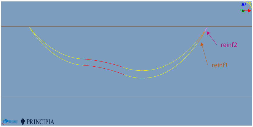
Figure 3 : Oil offloading lines shape.

Model Excel Datasheet

In the following slides, the main steps of the model setup are described in interactive mode.

The file ModelXls_CALM_BUOY_EXAMPLE.xlsx is provided in DeepLines WIND installation folder. This Model DataSheet contains several tabs, each corresponding to a panel that can be opened interactively via the graphical interface.

The DataSheet can be opened through the GUI or simply dragged and dropped into it if the GUI is already running. The tab named 'General' is used to include information about the model and to define the main input data, which directly populates certain cells in the Model DataSheet.

If needed, users can add additional tabs with specific names (such as INPUT_DLC in our example) to keep track of the original input data on which the model is based. These tabs will be ignored when the model is loaded.

If there are inconsistencies in the model definition during loading, the process will be stopped, and error messages will be displayed on screen and saved in the file LOG_History.txt.

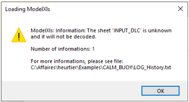
Figure 4 : Once user drag and drop xslx file, a message appears in GUI.

Note

For more details about the creation of a Model DataSheet please refer to “EX01-DLW_Jacket_ModelDataSheet_Tutorial.pptx”

Coupled Anaysis

For a CALM buoy, coupled analysis are required (at least to get the RAOS of motions):

• The buoy DOF are added into the global system

• Capture the interactions between the buoy and the lines, especially the dynamic part of the mooring lines and the Offloading lines

\[ (M + M_a(\infty)) \ddot{X}_{HF}(t) + \int_{0}^{t} R(t - \tau) \dot{X}(\tau) \, d\tau + K_{hyd}(t, X) X_{HF}(t) = F_{wind}(t, X) + F_{cur}(t, X) + F_{Drag}(t, X) + F^{(1)}_{wave}(t, X) + F_{Mooring}(t, X) + F^{(2)}_{IncidentWave} \]

• X: position of the floater (6DOF)
• Radiation loads are function of wave period (retardation function)
• FWave deduced from exciting loads
• Fdrag+Fwind+Fcur: viscous efforts due to wind / water relative velocity
• Fmooring restoring mooring/risers forces
• 2nd LF incident wave loads

Depending on the project phase and constraints, the RAOs of motions may be used as input data for uncoupled analysis, especially for the OOLs design phase

CALM buoys are floaters of intermediate size and can be modelled in different ways. The modeling approach presented here follows the conclusions of the JIP « CALM Buoy » led by PRINCIPIA in 2001-2005 • The buoy is seen as a hydrodynamic « large body » • A specific attention shall be paid to the viscuous damping : even if the use of damping matrices (P1/P2) may be correct for smaller buoys (OD<20m), the introduction of local drag elements in relative velocity shall be privilegied

-	POTENTIAL	POTENTIAL WITH DRAG
MODEL	Single rigid floater	Single floater with rigid drag elements
LOADING	Potential Flow (i.e diffraction/radiation)	Potential Flow +
Damping	Linear or Quadratic damping based on the CALM buoy motions	Damping on local elements based on relative fluid-structure velocity (cf References)

[1]. "JIP CALM Buoy Phase II: Model tests analysis report", RET.55.005.02, PRINCIPIA

[2]. "Component Approach for Confident Predictions of Deepwater CALM Buoy Coupled Motions – Part 1: Philosophy", OMAE2005-67138

[3]. "Component Approach for Confident Predictions of Deepwater CALM Buoy Coupled Motions – Part 2: Analytical Implementation", OMAE2005-67140

[4]. "JIP CALM Buoy Phase II: Buoy damping formulation – Specification document", DSL.55.080.01, 23/02/2005

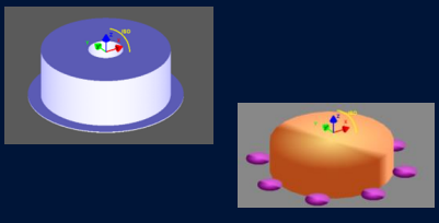
The modeling process requires the input of the hull’s mesh, which serves as the foundation for the structural and hydrodynamic analysis. An iterative workflow is then carried out between the mechanical model and the HDB (HydroDynamic Behavior) module to ensure consistency and convergence of the coupled system. This loop allows for refinement of the model by continuously updating the interaction between structural responses and hydrodynamic forces.

STEPS	DLW Model	HDB Creation Module
STEP 1: 1st order wave loads	• Define a Generic Floater • Import a Mesh • Define a Floater motion type	• Launch 1st order diffraction/radiation • Generate the HDB file rev01
STEP 2: Complete model def.	• Update the floater motions options • Introduce own Mass and Inertia terms • Introduce the viscous damping • Create the Buoy mooring lines & the Offloading system • Define a Frequency Domain(*) • Check it runs fine
STEP 3: Motions RAOs		• Select the FD analysis for the RAOs motions computation • Update the HDB file in rev02 (incl. Motions RAOs)
STEP 4: 2nd order wave loads		• Update the HDB file with the 2nd order wave loads • Update the floater motion type with HDB rev03
STEP 5: Complete Analysis	• Define your DLCs They may be coupled or uncoupled in FD or TD

Note

• Different set of motions RAOs (different HDB files) can be created deending on the wave introduced in the FD analysis.
• If an irregular wave spectrum is used, the stochastic process will be used for linearize the drag quadratic terms.

STEP 1: Define a Generic Floater and import a Mesh

STEPS	DLW Model	HDB Creation Module
STEP 1: 1st order wave loads	• Define a Generic Floater • Import a Mesh • Define a Floater motion type	• Launch 1st order diffraction/radiation • Generate the HDB file rev01

STEP 1 : 1st order hydrodynamic data:

• Create a “Generic floater” in a DSK, give it a name “Ex_buoy_hdb_creation.dsk”
  

• Define a reference node position which will be the reference position of your floater in the 3D scene
  

In this example, the reference node is the mid buoy and MSL when the draft is 6m.

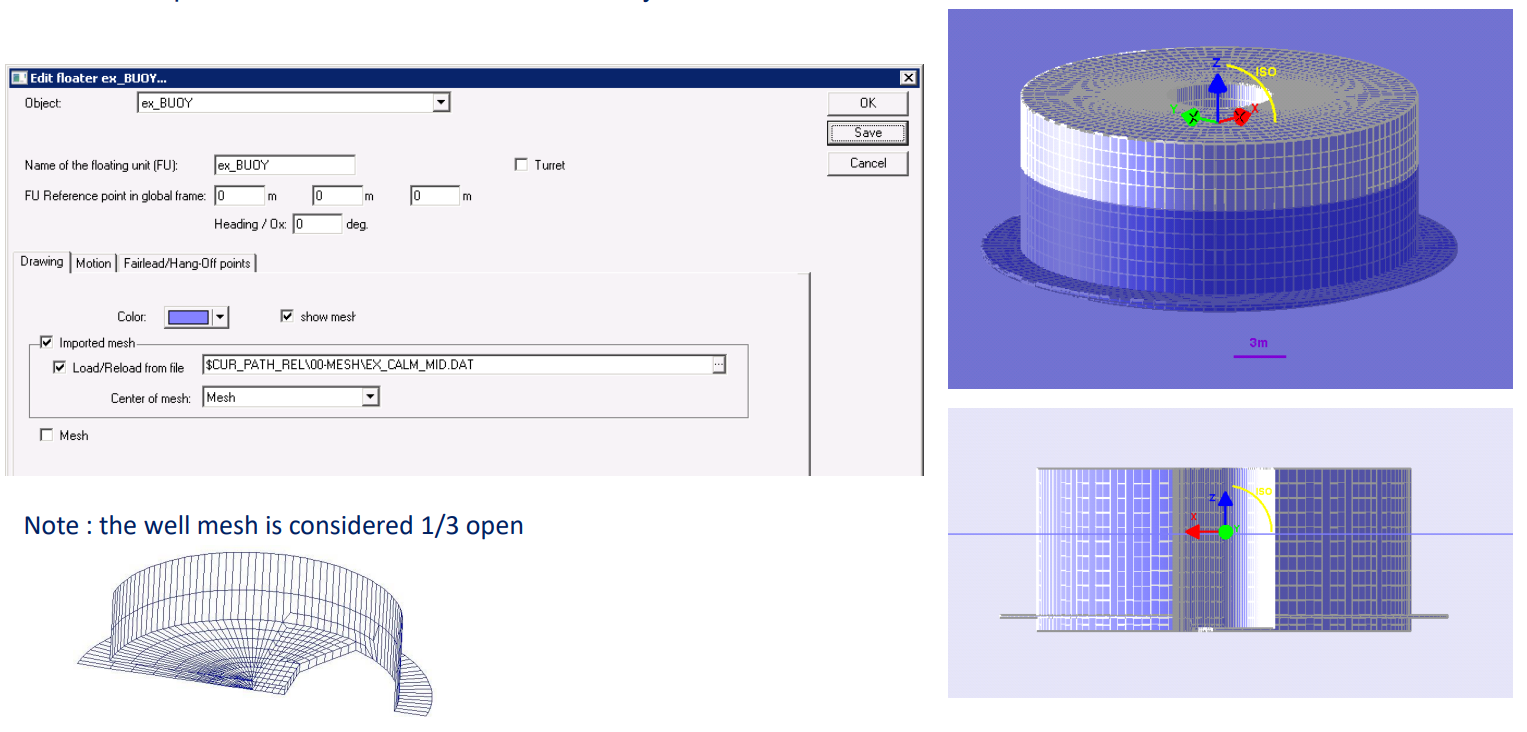
Figure 5 : Association between mesh and the generic floater.

Tips:

• As a fist step, only half of the buoy mesh is used to take advantage of the symmetry.
  

• This reference node is not necessary the same as the mesh reference, you can choose the most convenient reference node for the global model.
  

• Here, the mesh refers to the keel centre and a specific Buoy fairlead is created, named « mesh » with local coordinates wrt the reference point : (0, 0, -6)
  

• It is highly recommended to use $CUR_PATH_REL to define the path to the mesh file, this may make much easier any transfer of your model to another folder provided you respect the same architecture.
  

• $CUR_PATH is defined in the global settings; $CUR_PATH_REL is based on $CUR_PATH, « _REL » is useful anytime a file is needed both by the interface and the solver. In that case, when the input LOG file is generated, $CUR_PÄTH_REL replaced by « .. »
  

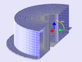
Figure 6 : Buoy mesh.

For instance, in the figure below here « $CUR_PATH » refers to the $Path\Examples\CURRENT_FOLDER and for every analysis, the solver will create a specific folder using the analysis name :

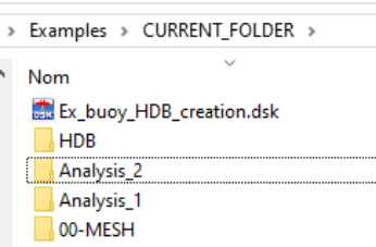
Figure 7 : Mesh Path.

Note

Folder « HDB » is the default folder automatically generated by the HDB creation module**

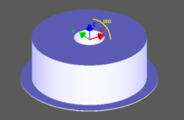
Define a preliminary floater motion type

A default “floater motion” type is automatically created and linked to the generic floater during the setup process. At this stage, the key parameter to define is the Center of Motion, which determines the reference point for evaluating hydrodynamic behavior within the HDB module. This definition is crucial for accurate motion modeling and ensures consistency in the dynamic response calculations.

Note: In the HDB, this centre of motion will be named [CENTER_OF_GRAVITY] for historical reason, even if it is not the real COG

By default, the centre of motion is the global reference node but any node can be chosen.

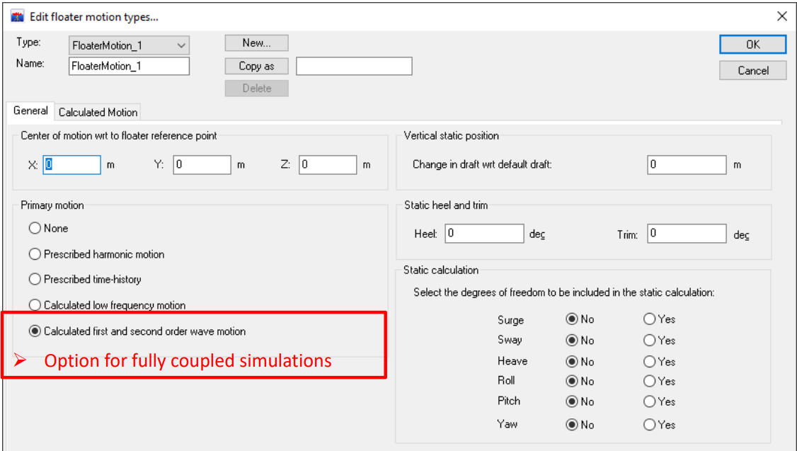
Figure 8 : Option for fully coupled simulation.

Launch 1st order diffraction/radiation and Generate the HDB file rev01

Open HDB Creation window

• Select your generic floater
  
• You can modify the range of periods / headings (for the first time, we recommend making a first quick tests with only 3 periods (require minimum) and one heading).
  
• Click on “Create files”
  
• The input file (.INP and the mesh file .DAT) for DIODORE module may be created and modified if needed to define symmetry axis
  
• Click on “Calc HDB” (for the first time, do it interactively but after it is better to use the batch mode (with Gen Batch file) since the hydrodynamic module may take some time to run.
  Note : Of course, if the INP has been modified at step c) , it should not be overwritten.
  
• Wait for “End of Generation”. You can check that a folder “HDB\Floater_name” has been created and inside you have your HDB file
  

--> Check the [STRUCTURE_01] name, this will be needed in the floater motion property (next step)

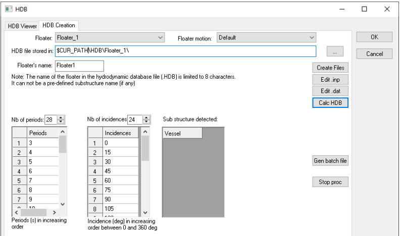
Figure 9 : HDB creation window.

Tips for Symmetrical Mesh

For symmetrical mesh, it is possible to import only a part of the total mesh

When the *.INP file is created, the following keywords must be added:

• Single plane symmetry with respect to the plane [y = 0]: *SYMMETRY,NAME=SYMD,COORD=Y
  

• Double plane symmetry with respect to planes [x = 0] and [y = 0]: *SYMMETRY,NAME=SYMD,COORD=XY
  

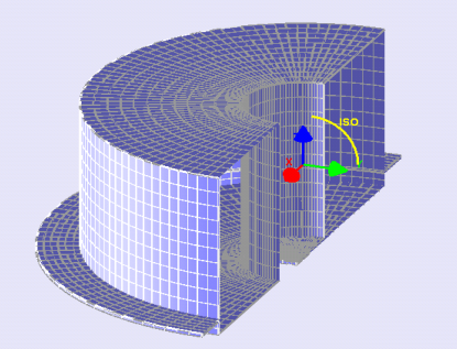
Figure 10 : Symetrical buoy. INP modification.

End of Step 1 and Resulting HDB file rev01

At the end of step1, the HDB file provides some of the terms of equations of Buoy motions :

\[ (M + M_a(\infty)) \ddot{X}_{HF}(t) + \int_{0}^{t} R(t - \tau) \dot{X}(\tau) d\tau + K_{hyd}(t, X) X_{HF}(t) = F_{wind}(t, X) + F_{cur}(t, X) + F_{Drag}(t, X) + F^{(1)}_{Wave}(t, X) + F_{Mooring}(t, X) + F^{(2)}_{IncidentWave} \]

\( M_{a}(\omega)\ddot{X}_{H/F}(t) + \int_{0}^{t} R(t-\tau)\dot{X}(\tau)d\tau \)	Added mass Radiation damping matrices at section [Added_mass_Radiation_Damping] in HDB file. The second term is often reported as the "memory effect".
\( F^{(1)}_{\text{wav}}(t,X)+ \)	The wave first order excitation loads are given in three different sections in the HDB file: - section [FROUDEKRYLOV_FORCES_AND_MOMENTS]: includes only the incident wave load components - section [DIFFRACTION_FORCES_AND_MOMENTS]: includes only the diffracted components - section [EXCITATION_FORCES_AND_MOMENTS]: includes the sum of all components Note: When the non-linear Froude-Krylov option is selected, only the second component is read from the HDB. The FK components are computed during time simulation in DLW.
\( K_{\text{hyd}}(t,X)\dot{X}_{H/F}(t) \)	The hydrostatic matrix is due only to buoyancy efforts, since no inertia has been defined yet. This term will be ignored because the non-linear hydrostatic option will be used after Step 2, and the complete hydrostatic matrix will be recomputed by DLW.

STEP 2 : Complete Model Definition

STEPS	DLW Model	HDB Creation Module
STEP2: Complete model def.	- Update the floater motions options - Introduce own Mass and Inertia terms - Introduce the viscous damping - Create the Buoy mooring lines & the Offloading system - Define a Frequency Domain - Check it runs fine

Floater motion update

• At the end of STEP1, a HDB file has been created in the working directory of the HDB creation module

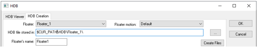
Figure 11 : Working directory HDB folder.

• In DeepLines model, the floater motion property is updated:

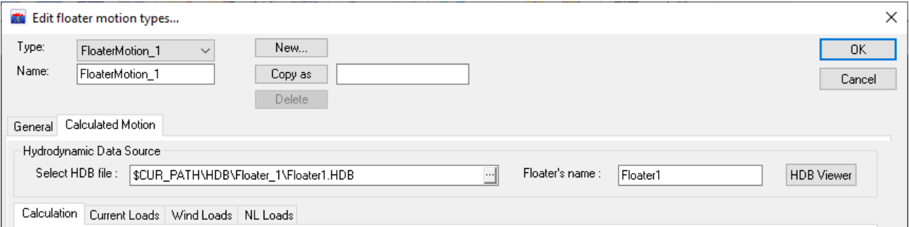
Figure 12 : Floater motion type property update.

• If a reduced mesh is used at step 1, the complete hull mesh shall be now introduced for the non-linear hydrostatic and Froude-krylov option.

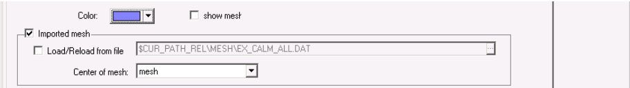
Figure 13 : Check whole mesh.

The Buoy motion property may be updated through:

• First order wave loads

• Non-linear & Froude Krylov loads

• Viscous drag damping

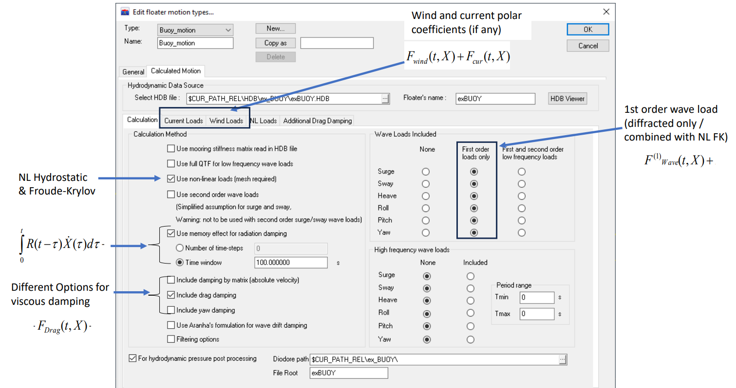
Figure 14 : Floater motion type options to select.

Buoy own Mass and Inertia terms

Buoy mass and inertia are introduced as a lump mass on a specific Buoy fairlead representing the center of gravity

In this example, the centre of gravity is centered at 0.17m above the selected reference (MSL)

Note

If needed, the inertia terms can be completed with an inertia matrix but be carefull, pure inertia terms generate no weight.

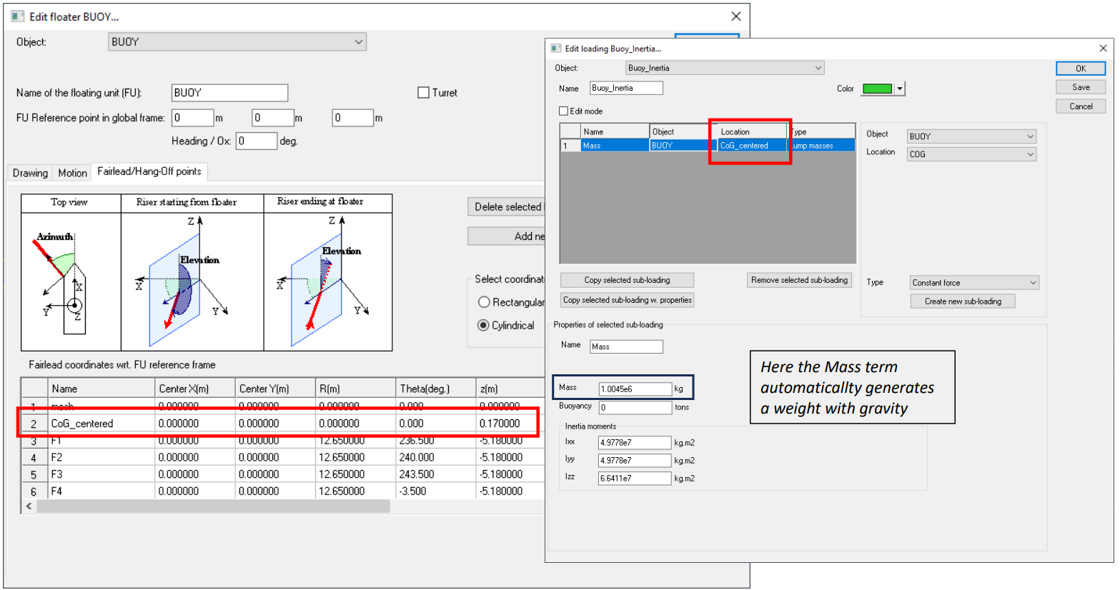
Figure 15 : Add loading to consider buoy mass and inertia.

Buoy viscous damping

Buoy Viscous damping is defined with specific bar elements using a Morison type formulation.

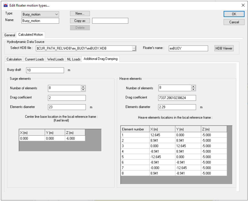
Figure 16 : Addional drag damping.

In DLW, the Morison reference area is calculated as the product of the element’s outer diameter (OD) and its total length (L), which is the sum of all drag elements. For surge motion, L corresponds to the buoy draft; however, for high wave conditions, it is recommended to use the buoy height to ensure drag is integrated over the entire immersed portion of the buoy body. In this case, OD refers to the buoy body, and a drag coefficient (Cd) of 2 is typically applied. For heave and pitch motions, DLW automatically generates small elements with a fixed length of 0.02 m. Their outer diameter and axial drag coefficient (CD_ax) should be adjusted accordingly to match the desired reference damping.

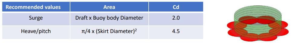
Taking, OD = 0.5*(OD_skirt – OD_body), it comes:

Surge Damping Elements	Value
OD	23 m
Length	10 m
CD	2 SI

Heave/Pitch Elements	Value
OD	2.290 m
Length	0.02 m
CD_axial	7337.29 SI

Buoy mooring lines and fairleads

Definition of the Buoy Mooring Lines :

▪ Create Buoy fairleads

Legs	Azimuths (deg)
1, 2, 3	236.5, 240, 243.5
4, 5, 6	-3.5, 0, 3.5
7, 8, 9	116.5, 120, 123.5

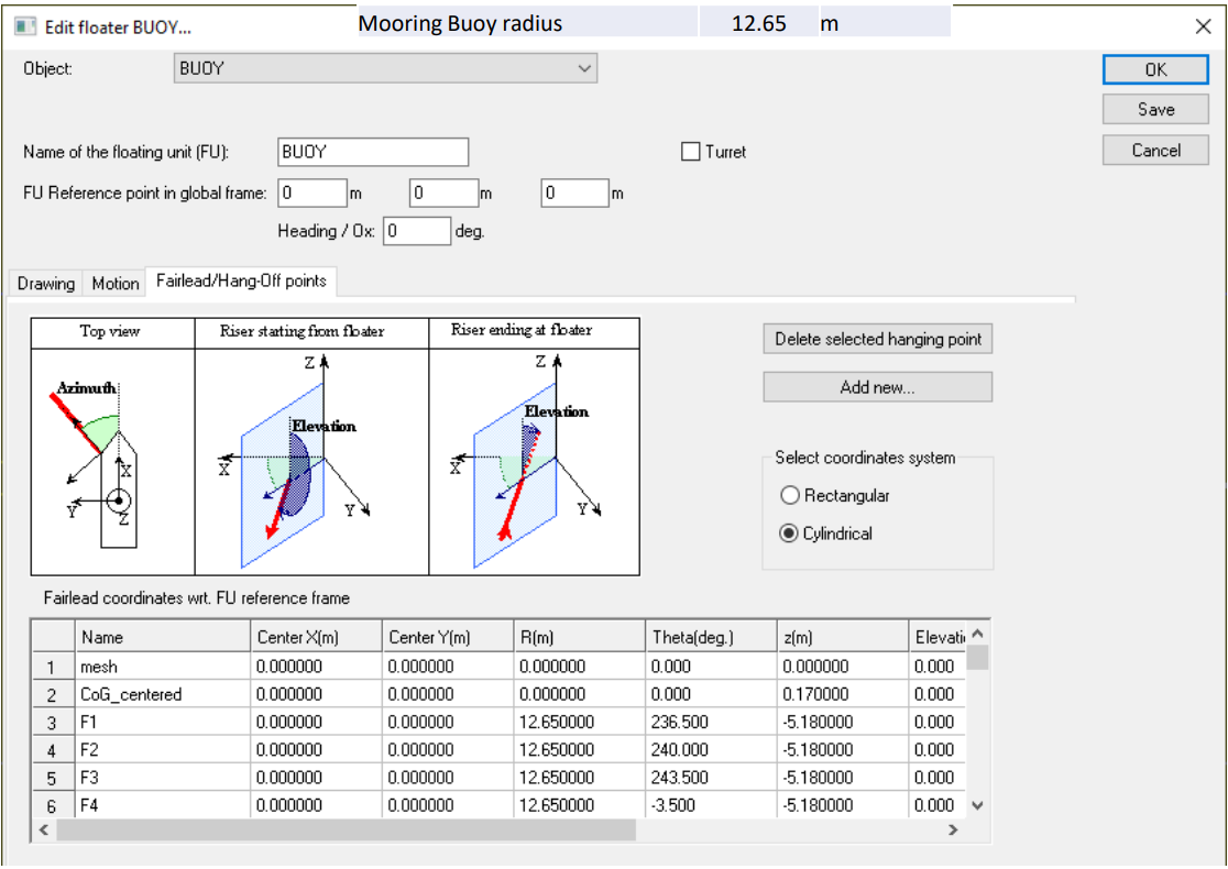
Figure 17 : Buoy fairleads.

Create anchor points in “Sea & ground” panel :

• Environment : view and size of the 3D scene for the global model

• Physical parameters : density, viscosity and gravity and sea water depth

• Sea bed shape : horizontal / flat with slope / user defined with mesh) and position

• Ground connections (Here it is easer to use “cylindrical coordinates)

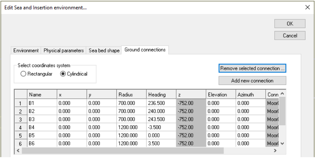
Figure 18 : Achors positions.

Buoy mooring lines

Mooring lines properties :

• Lines properties : Create a “cable/chain type” for each segment

Note

• Cable/chain are modelled as bar or cable elements as bending/torsion is ignored

• For OPB/IPB problems, beam elements shall be used

• Specific properties can be defined (non-linear / synthetic or Constitutive law) which are not addressed in this example

• For hydrodynamic coefficients for chain, the hydrodynamic diameter to consider is 1.8 times the link diameter.

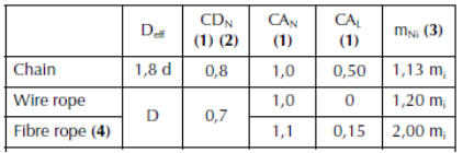
Table 2 : Hydrodynamic coefficients

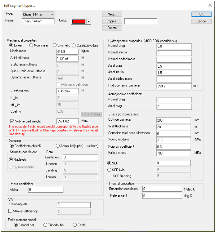
Figure 19 : Chain type properties.

Lines definition

For each Mooring line: Create a generic line and Double click on the new line “GenLine_1” in model to edit it.

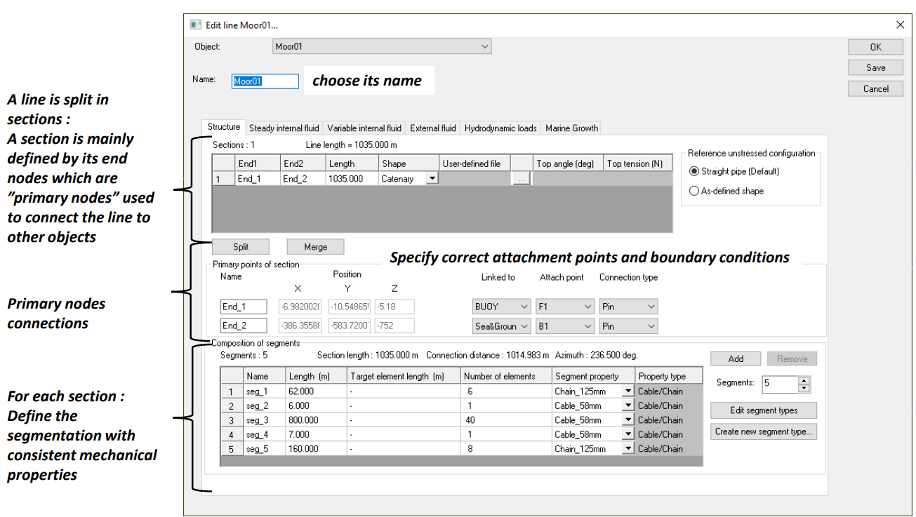
Figure 20 : Mooring lines segmentation.

Offloading system

For OOLs, the same steps are conducted except that OOLs are defined as beam elements.

As they are rigid pipes, different « rigid types » properties are used for the standard segments, the reinforced ones as well as the buoyant segments.

In the next image, every property is associated with a color:

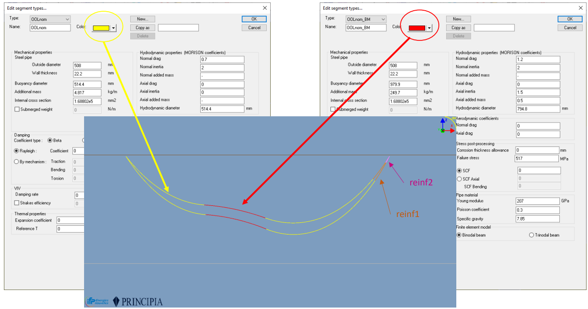
Figure 21 : OOL lines type.

Every OOL is connected on one end to the FPSO and on the other end to the Buoy.

The only specific point to mention is the flexjoint connection on the buoy side.

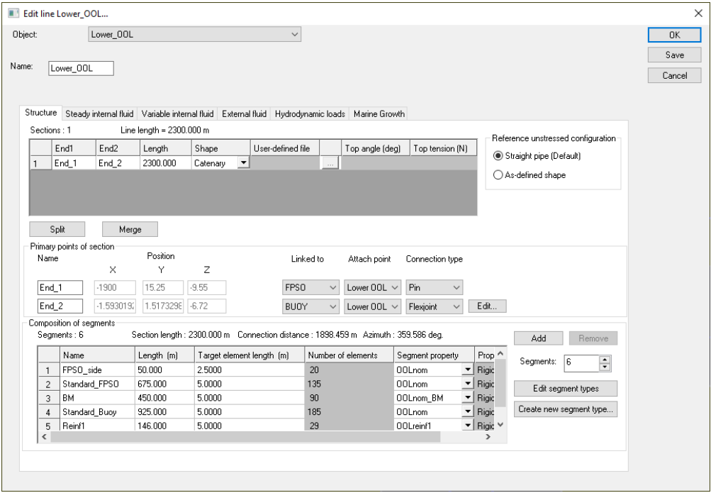
Figure 22 : OOL segmentaiton.

OOL internal fluids

OOLs are filled with Oil content with a density of 0.931. A design pressure of 30 bars is considered for post-processing only that means that we choose here not to consider the end cap effect during the simulation.

On FPSO side, the hydrostatic pressure corresponds to 9.55m of Oil density below the MSL at the FPSO fairlead. The hydrostatic pressure will be updated along the OOLs considering the vertical position at each arc length wrt the FPSO fairlead.

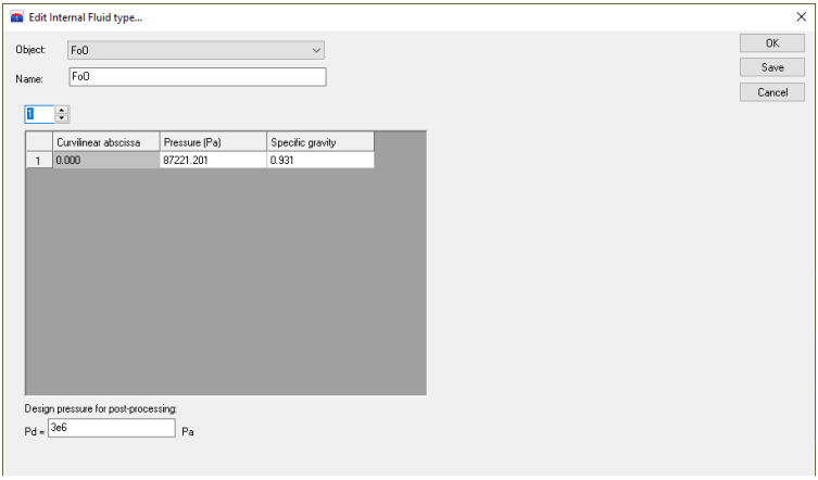
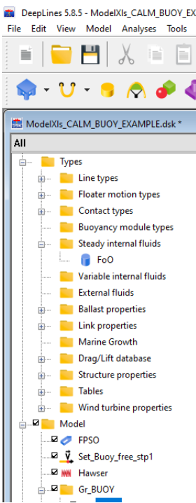
Figure 23 : OOL internal fluids.

TurnTable and Hawser Setup

In this example, a hawser is introduced and connected to a turntable fixed on the buoy, which may be set free to rotate.

To achieve this, a rigid body named TurnTable is defined and connected to the buoy axis using two stiff springs.

The hawser is connected on one side to the top of the buoy turntable, located 7 meters from the buoy center.
On the other side, it is intended to connect to a tanker, which is not defined here.

The hawser is oriented in the opposite direction to the Oil Offloading Lines (OOLs) and is clamped.

For visualization purposes, a frame of "fake" bars is attached to the turntable using an external mesh file.
This mesh is not used for computations.

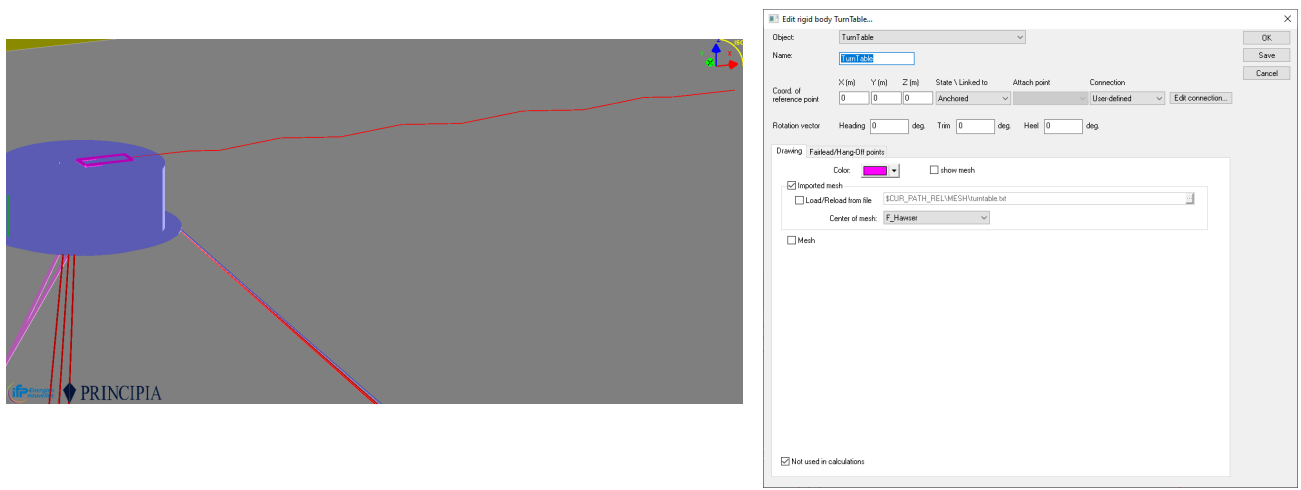
Figure 24 : Turntable as a rigid body not used in calculation.

The hawser is seen as a spring with a multi-linear law. The global weight of 1800kg is considered at the turntable connection.

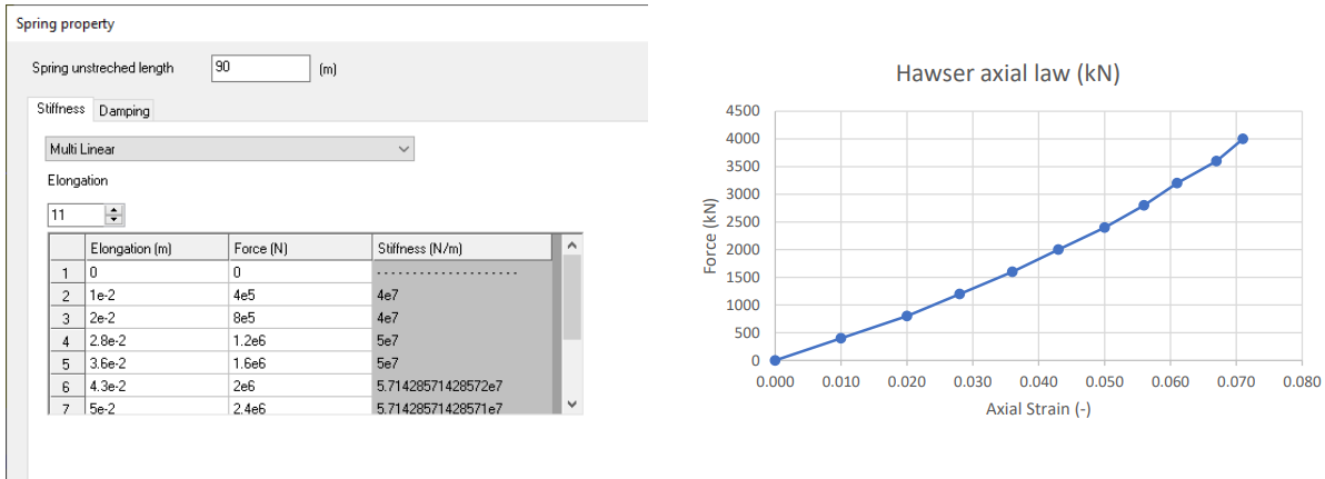
Figure 25 : Define hawser properties as a spring with multi-linear law.

Ballast definition

An excentric liquid ballast is added to counteract the moment induced by the tensions of anchoring lines opposite to the OOLs.

To do so, a Ballast object is used with a filling ratio of 100%, with the following property:

Parameter	Unit	Value
Ballast weight	t	254.5
Volume	m³	248.29
Length	m	6
Equivalent Outer Diameter	m	7.26
Location w.r.t buoy center	m	7.875
Azimuth	deg	185.5
Elevation (above keel)	m	3.97

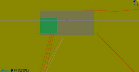
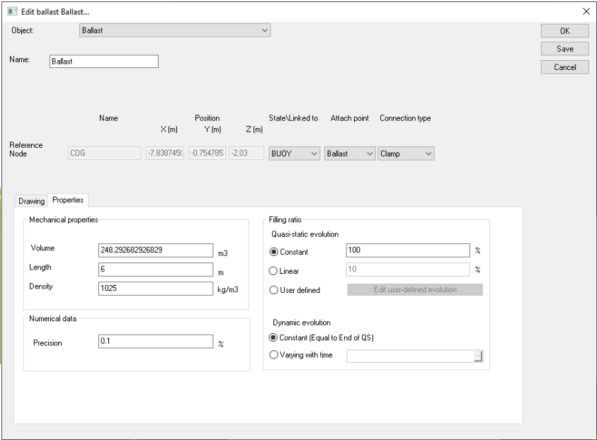
Figure 26 : Buoy ballast.

Static check

Before going further, it is recommended to perform a first static check.

To do so, proceed as such: - In “Default” folder create a new analysis - Give it a name, for instance “Check_stat” - Edit the analysis and select the objects that will be part of it - Define only a static analysis with step 0 and step 1

Note

In the example below, the hawser is not included (Idle Buoy case) and a specific displacement named “Set_Buoy_free_stp1” is used to set the buoy free at the quasi-static step 1. Please ref to “D4 - L5 - DeepLines Wind - playing with DOF.pdf” for more details.

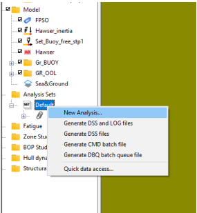
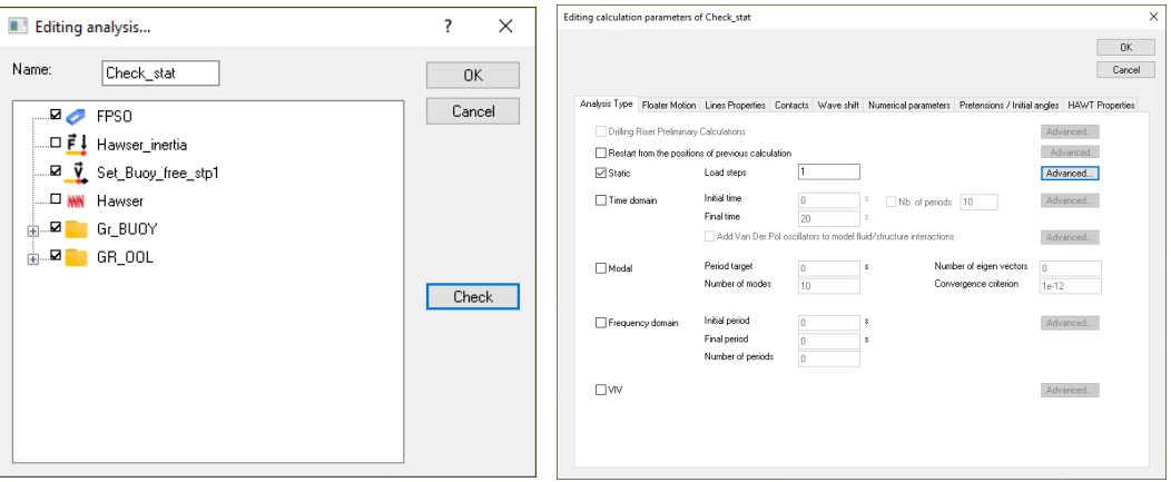
Figure 27: Check static.

During the computation, a file *.DAY is created giving information about the Buoy at the end of step 1.

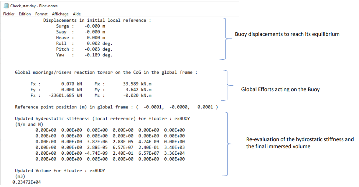
Figure 28: Check static analysis .day file.

Of course, other results may be requested in the DSS file post-processing.

Definition of a Frequency Domain and checks

At the end of step 2, a frequency domain analysis is defined which will be used to compute the RAOs of motions.

• Copy “Check_stat” and rename it “FD_RAO”.
  

• Add a wave to select the type of wave as well as the wave height for which the RAOs are to be computed.
  

• Here, a unitary regular wave (H=1m) going to the X axis (heading = 0deg).
  

• For checking purpose, the selected periods range is [3,20]. In any case, this will be automatically adjusted by the HDB module to the number of periods already computed in the HDB file.
  

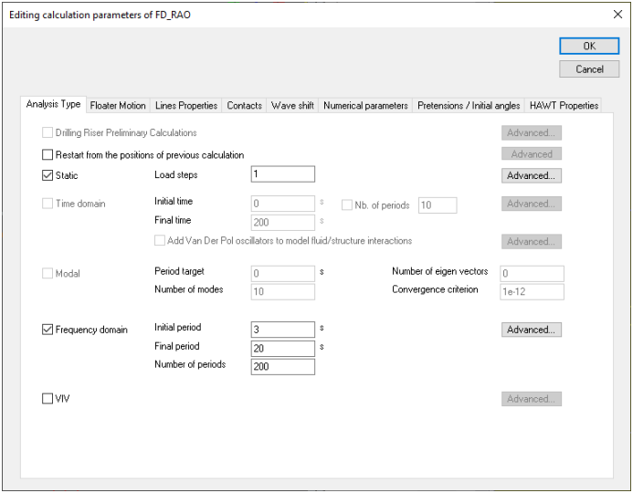
Figure 29: Frequency analysis.

For a wave heading at 0 deg, the surge, heave and pitch RAOs are post-processed.

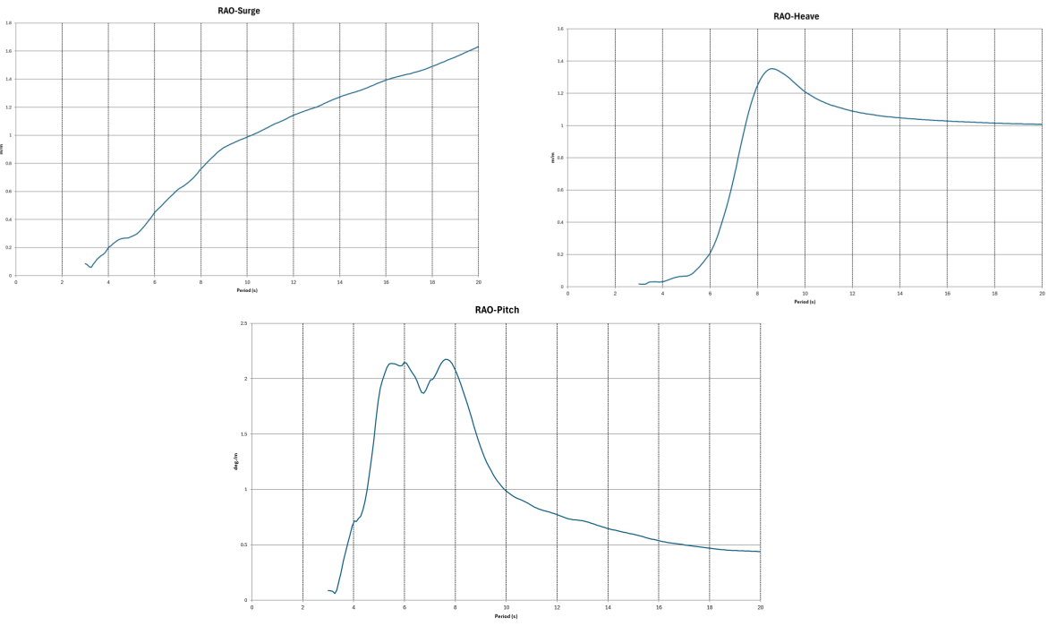
Figure 30: Post processing : RAO surge, heave and pitch.

Even if the studied offloading system is different, the motions RAOs are consistent with the RAOs provided in Paper No: 2007-JSC- 594 “Derivation of CALM Buoy Coupled Motion RAOs in Frequency Domain and Experimental Validation” .

RAOs of tension for one mooring line and the axial plus bending stress at both OOL buoy ends are also post-processed. It can be highlighted that the buoy motions greatly impact the RAOs of OOLs stresses and mooring tensions.

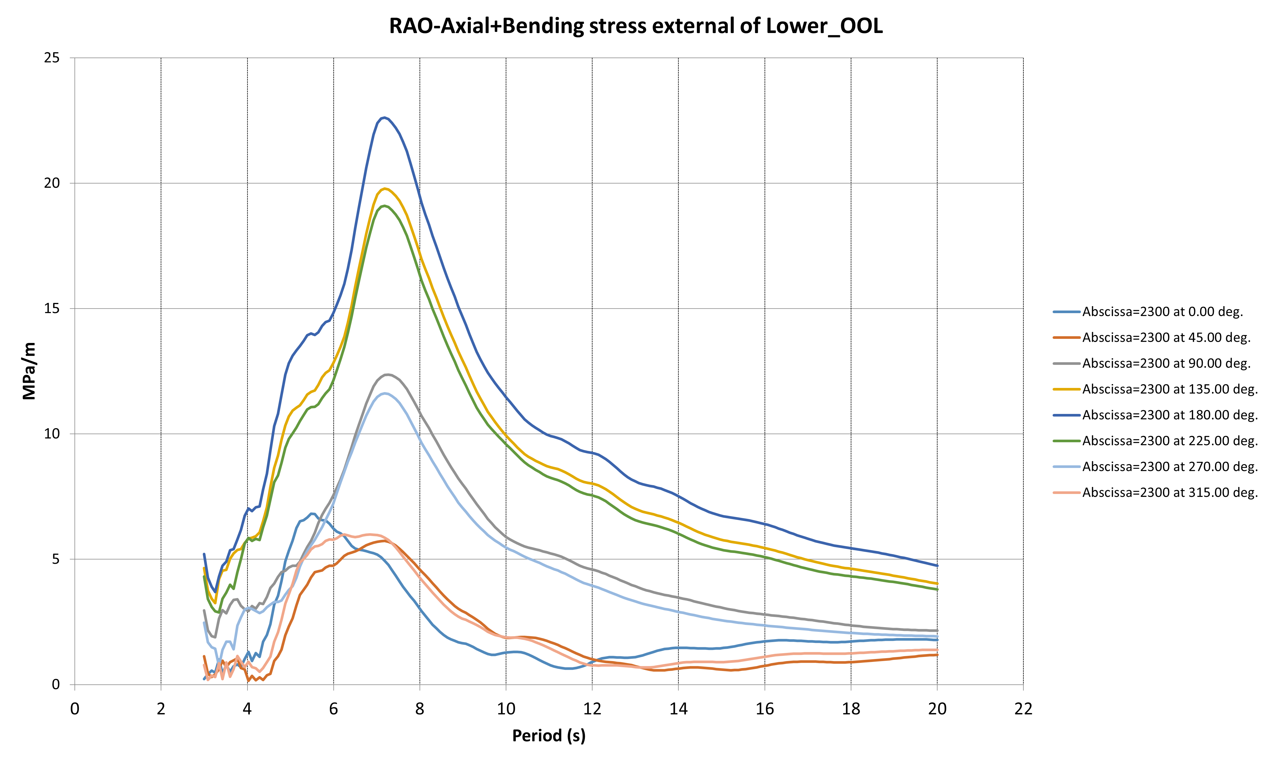
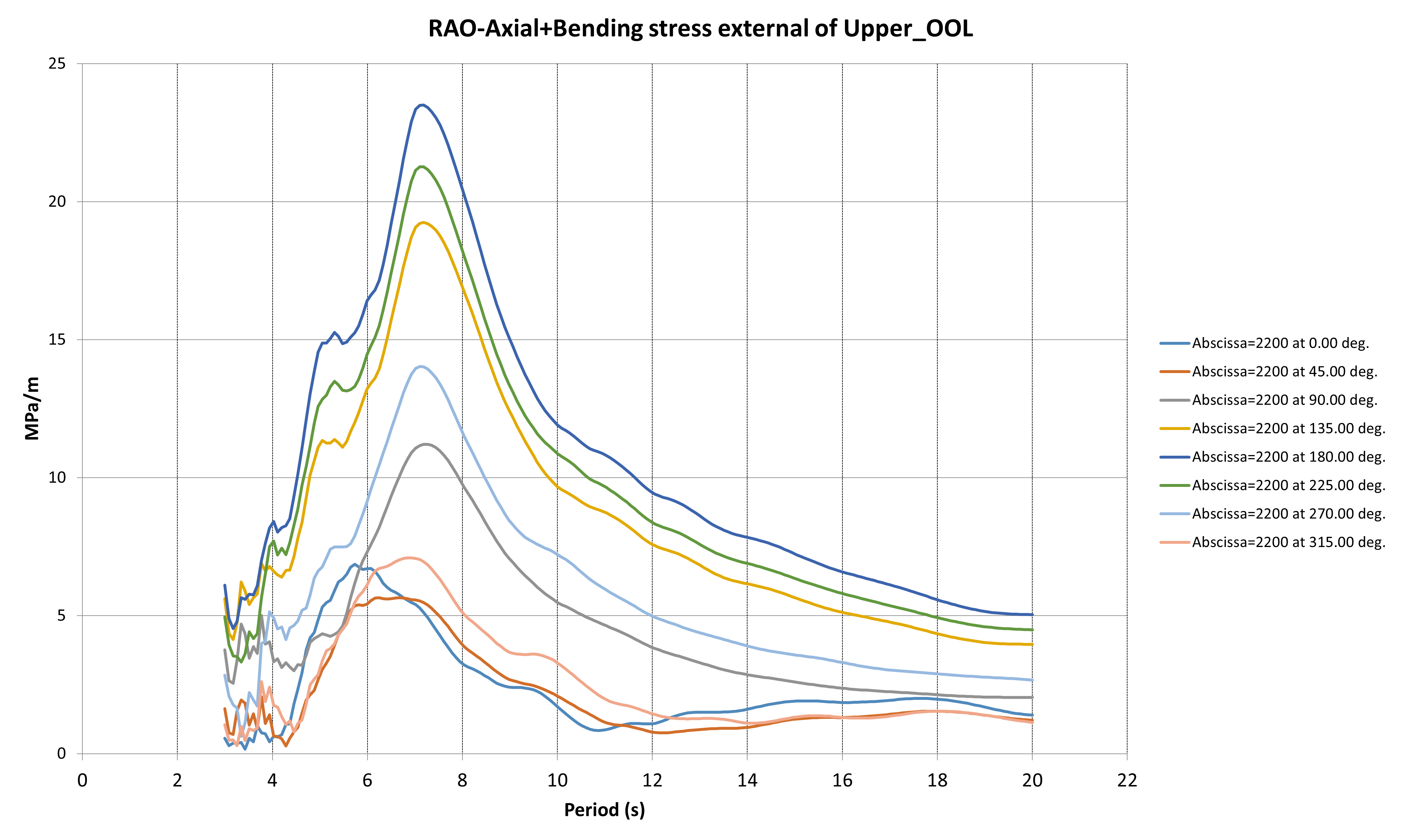
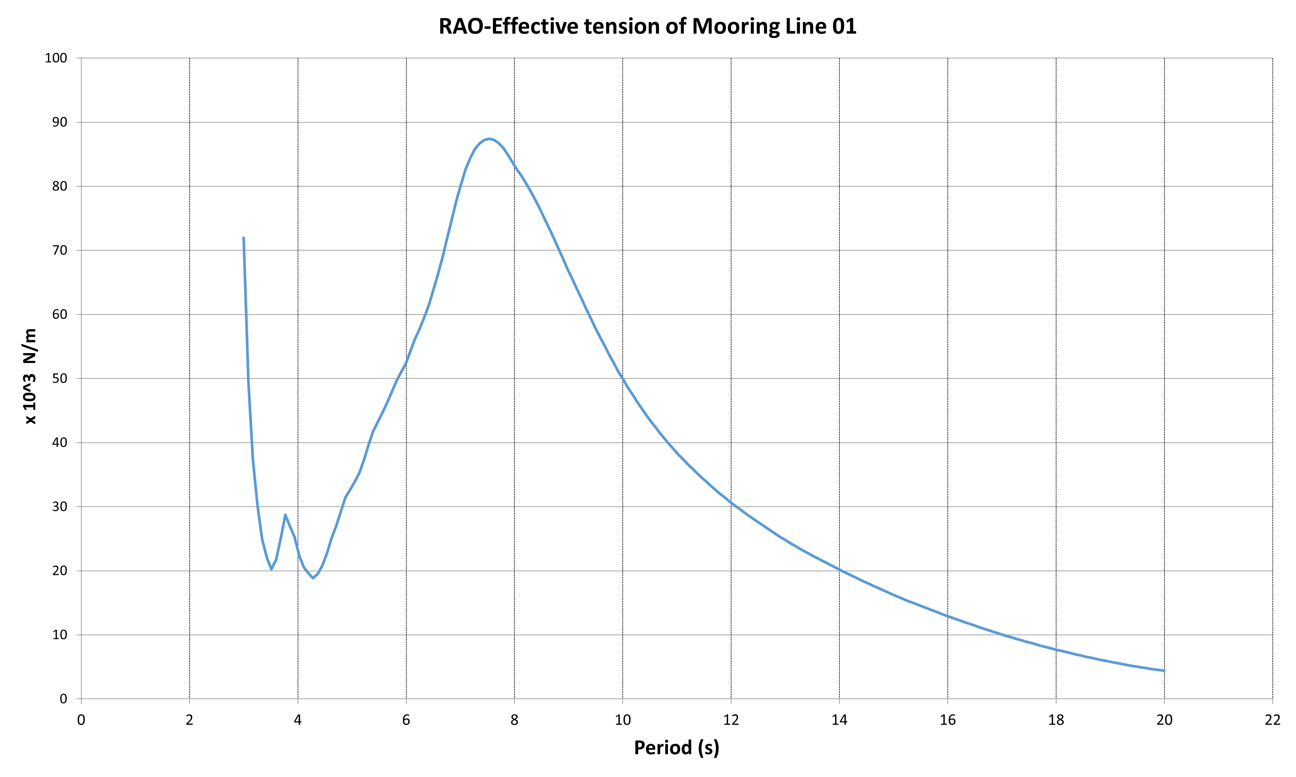
Figure 31: Postprocessing : stress RAOs.

STEP 3 & 4 : Update of HDB file with motions RAOs

Select the FD analysis for the RAOs motions computation and update the HDB file (with or without 2nd order loads)

STEPS	DLW Model	HDB Creation Module
STEP 3: Motions RAOs		- Select the FD analysis for the RAOs motions computation - Update the HDB file in rev02 (incl. Motions RAOs)
STEP 4: 2nd order wave loads		- Update the HDB file with the 2nd order wave loads - Update the floater motion type with HDB rev03

Coming back to the HDB creation module:

• Step 3: The HDB file can now be updated with motions RAOs computed with the whole mechanical system. This HDB can then be used for uncoupled analysis, for instance fo the OOLs design.

• Step 4 : The HDB file can be updated with the second order loads which depend on the motion RAOs.

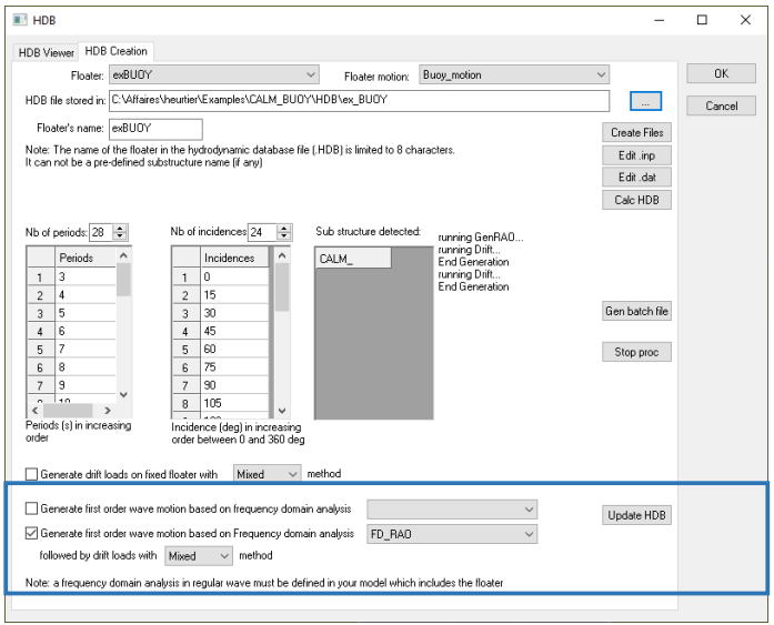
*Figure 32: Update HDB file with frequency analysis results. *

Update the floater motion type

Finally, the floater motion property must be updated depend on the type of analysis to be performed.

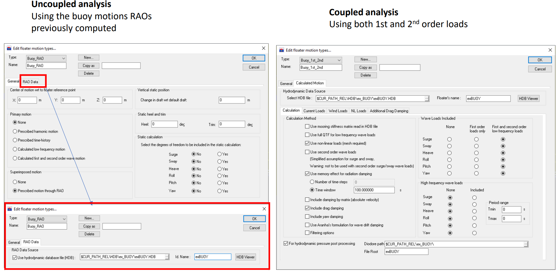
Figure 33: Options to select depending on analysis user wants to perform.

STEP 5 : Example of fatigue DLC

STEPS	DLW Model	HDB Creation Module
STEP 5: Complete Analysis	- Define your DLCs They may be coupled or uncoupled in FD or TD

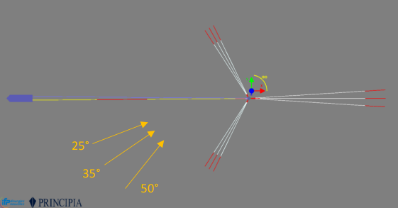
Figure 34: Wave heading for DLW matrix.

A fatigue analysis of the OOls is performed considering three main directions for the sea-sates. Jonswap Spectra are considered with a gamma coefficient of 2.

Fatigue Analysis - Input Data

Wave Energy Distribution – Direction 25°

Hs (m)	Tp = 2s	Tp = 4s	Tp = 6s	Tp = 8s	Tp = 10s	Tp = 12s	Tp = 14s	Tp = 16s	Tp = 18s	Tp = 20s	Tp = 22s	Tp = 24s	Tp = 30s	Tp = >0s
0.25	0	0	0	0.0237	0.1437	0.0712	0.1200	0.0475	0.0237	0	0	0	0	0.43
0.5	0	0	0	0	0.6685	3.3901	2.4354	1.0746	0.4536	0.0712	0	0	0	8.09
0.75	0	0	0	0	0.5248	4.7746	4.4410	1.3133	0.4773	0.0712	0	0	0	11.60
1.0	0	0	0	0	0.2149	1.7669	4.6321	1.6232	0.1437	0.0237	0	0	0	8.40
1.25	0	0	0	0	0	0.7397	2.5066	0.6448	0.0950	0.0237	0	0	0	4.01
1.5	0	0	0	0	0	0.2862	1.1696	0.5486	0.0950	0.0237	0	0	0	2.12
1.75	0	0	0	0	0	0.1437	0.5011	0.3336	0.0475	0	0	0	0	1.03
2.0	0	0	0	0	0	0.0237	0.0475	0.2149	0	0	0	0	0	0.29
2.25	0	0	0	0	0	0	0	0.0237	0	0	0	0	0	0.02
2.5	0	0	0	0	0	0	0	0	0	0	0	0	0	0.00
2.75	0	0	0	0	0	0	0	0	0	0	0	0	0	0.00
3.0	0	0	0	0	0	0	0	0	0	0	0	0	0	0.00
3.25	0	0	0	0	0	0	0	0	0	0	0	0	0	0.00
3.5	0	0	0	0	0	0	0	0	0	0	0	0	0	0.00
3.75	0	0	0	0	0	0	0	0	0	0	0	0	0	0.00
>0	0	0	0	0.02	1.55	11.20	15.85	5.82	1.34	0.21	0.00	0.00	0.00	36.00

Wave Energy Distribution – Direction 35°

Hs (m)	Tp = 2s	Tp = 4s	Tp = 6s	Tp = 8s	Tp = 10s	Tp = 12s	Tp = 14s	Tp = 16s	Tp = 18s	Tp = 20s	Tp = 22s	Tp = 24s	Tp = 30s	Tp = >0s
0.25	0	0	0	0	0.0947	0.0473	0.0237	0.0947	0.0473	0	0	0.0237	0	0.33
0.5	0	0	0	0	0.7610	2.8560	1.4760	1.6180	0.5468	0.0710	0.0473	0	0	7.38
0.75	0	0	0	0	0.3575	4.8788	4.6409	1.5233	0.1906	0.0473	0.0237	0	0	11.66
1.0	0	0	0	0	0.0947	2.2133	4.8066	1.1895	0.1906	0.0473	0	0	0	8.54
1.25	0	0	0	0	0	0.6427	2.3317	0.9516	0.1432	0.0710	0	0	0	4.14
1.5	0	0	0	0	0.0237	0.1906	0.9279	0.7137	0.1196	0.0237	0	0	0	2.00
1.75	0	0	0	0	0	0.0473	0.2379	0.2379	0.0947	0	0	0	0	0.62
2.0	0	0	0	0	0	0	0.0947	0.0473	0.0473	0	0	0	0	0.19
2.25	0	0	0	0	0	0	0	0	0	0	0	0	0	0.00
2.5	0	0	0	0	0	0	0.0237	0.0947	0	0	0	0	0	0.12
2.75	0	0	0	0	0	0	0	0.0237	0	0	0	0	0	0.02
3.0	0	0	0	0	0	0	0	0	0	0	0	0	0	0.00
3.25	0	0	0	0	0	0	0	0	0	0	0	0	0	0.00
3.5	0	0	0	0	0	0	0	0	0	0	0	0	0	0.00
3.75	0	0	0	0	0	0	0	0	0	0	0	0	0	0.00
>0	0	0	0	0	1.33	10.88	14.56	6.49	1.38	0.26	0.07	0.02	0.00	35.00

Wave Energy Distribution – Direction 50°

Hs (m)	Tp = 2s	Tp = 4s	Tp = 6s	Tp = 8s	Tp = 10s	Tp = 12s	Tp = 14s	Tp = 16s	Tp = 18s	Tp = 20s	Tp = 22s	Tp = 24s	Tp = 30s	Tp = >0s
0.25	0	0	0	0	0.1184	0.0469	0.0469	0	0.0234	0	0	0	0	0.2355
0.5	0	0	0	0	0.6128	1.3896	0.8717	1.1072	0.2121	0.0234	0	0	0	4.2168
0.75	0	0	0	0	0.5179	3.1330	4.0516	1.7669	0.2121	0.0234	0.0234	0	0	9.7283
1.0	0	0	0	0	0.1886	1.9087	4.9468	1.1775	0.3292	0	0.0234	0	0	8.5742
1.25	0	0	0	0	0.0469	0.6362	1.9555	1.1775	0.1886	0.0234	0	0	0	4.0282
1.5	0	0	0	0	0	0.2355	0.7299	0.5659	0.0703	0	0	0	0	1.6017
1.75	0	0	0	0	0	0.0234	0.2355	0.2355	0.0234	0	0	0	0	0.5179
2.0	0	0	0	0	0	0	0.0234	0.0703	0	0	0	0	0	0.0937
2.25	0	0	0	0	0	0	0	0	0	0	0	0	0	0.0000
2.5	0	0	0	0	0	0	0	0	0	0	0	0	0	0.0000
2.75	0	0	0	0	0	0	0	0	0	0	0	0	0	0.0000
3.0	0	0	0	0	0	0	0	0	0	0	0	0	0	0.0000
3.25	0	0	0	0	0	0	0	0	0	0	0	0	0	0.0000
3.5	0	0	0	0	0	0	0	0	0	0	0	0	0	0.0000
3.75	0	0	0	0	0	0	0	0	0	0	0	0	0	0.0000
>0	0	0	0	0	1.4845	7.3733	12.8614	6.1009	1.0591	0.0703	0.0469	0	0	28.9963

Fatigue analysis : DLC definition

Three Environment Sets are created combination for each direction all sea-states of the WSD and the motions conditions for the buoy (HDB file rev03) and the FPSO (fixed here).

Three Analysis Sets are then created based on every EnvironmentSet applied to the global system.

In this example, Frequency Domain simulations are defined that means that coupled analyses will be done with the whole system loaded by irregular waves. The Buoy motions will be computed using a stochastic linearization of damping.

For Time domain analyses, the same process is to be followed.

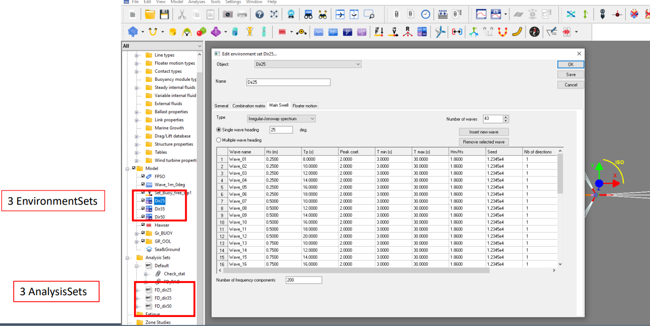
Figure 35: Environment set for fatigue matrix.

Fatigue Analysis : DLC runs

All simulations are run with the Batch tool, the number of simulations ran in parallel depends on the license key.

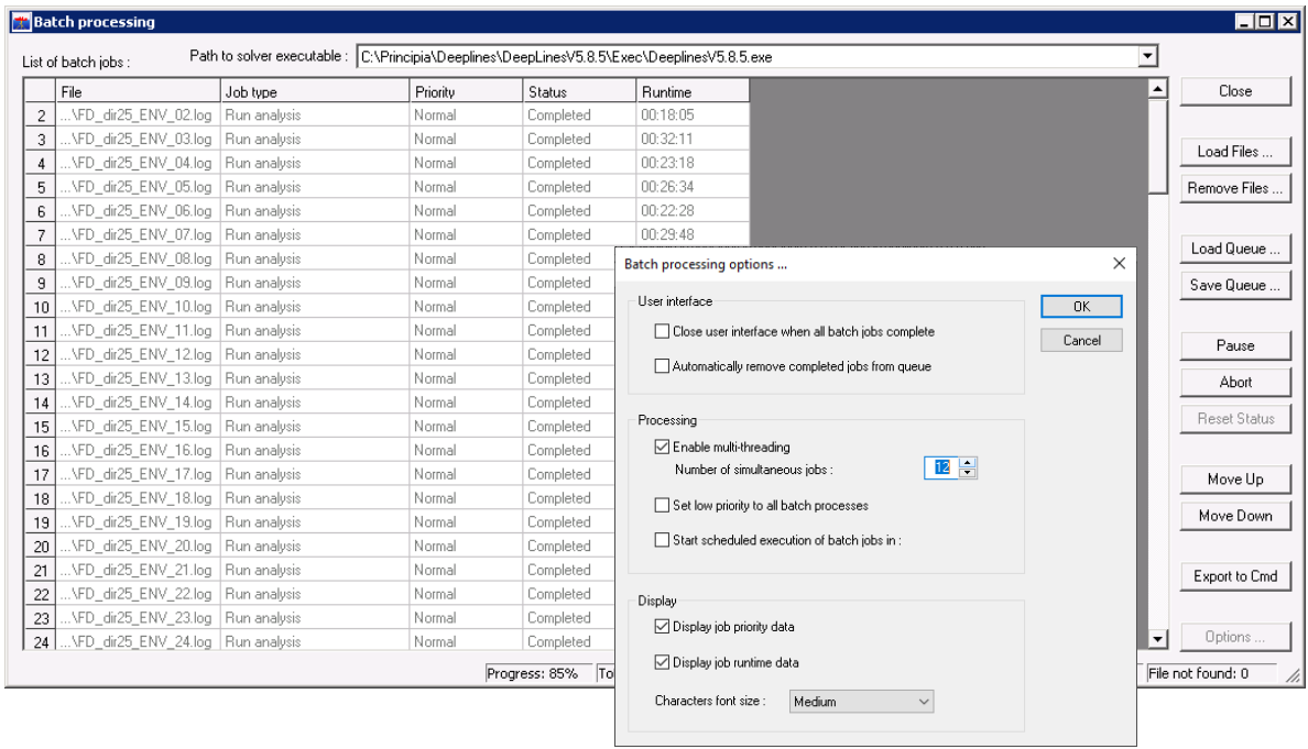
Figure 36: Batch processing, multi threading calculation.