Home > Theory > Contact Modelling > Pipe/Soil interactions
Pipe/Soil interactions
Table of Contents
1 Seabed Contact
1.1 Normal soil stiffness
1.2 Suction
2 Classical Approach for interaction curves
2.1 Context
2.2 P–y / T–z Curves
2.2.1 Concept Stage Practice
2.2.2 Spudcan Modeling Recommendations
2.3 Calculation method in DLW
2.3.1 The physics
2.3.2 In DLW
2.3.3 Input File Creation
2.3.4 Outputs
1. Seabed Contact
The seabed contact is ruled by so-called contact elements connecting a node of the riser with a node on the seabed. Following the relative positions of these two nodes, each contact element generates reaction and friction forces. It is important to note that the reaction forces are concentrated on the nodes.
The normal reaction force is proportional to the penetration \(\Delta Z\) except close to \(\Delta Z=0\) where a quadratic formula is used to ensure tangent continuity :
-
If \(\Delta Z \geq 0\) \(F_n = 0\)
-
If \(\Delta Z \lt 0\) then :
-
If \(\lvert\Delta Z\lvert \le \epsilon_Z\) then \(F_n= K_n \Delta Z^2/(2\epsilon_Z)\)
-
otherwise : \(F_n = -K_n(\Delta Z-\epsilon_Z/2)\)
where \(K_n\) is the normal contact stiffness and \(\epsilon_Z\) is tolerance on the penetration.
The nodal reactions must balance the apparent weight of all the elements connected to each node. For a binodal element, if \(L_0\) is the length and \(w_0\) its apparent weight, the nodal penetration is roughly be given by : \(\Delta Z = \frac{w_0 L_0}{2 K_n}\).
As for the lateral displacements, two friction coefficients are introduced along with two given directions \(u_1\)> and \(u_2\). The total friction force is \(F_{fric}=F_1+F_2\) and the Coulomb criteria is separately checked on both directions :
-
If \(\|F_1\| \leq \mu_1 F_n\) : \(F_1=K_{t1} \Delta x_1\) Otherwise \(F_1 = \mu_1 F_n u_1\)
-
If \(\|F_2\| \leq \mu_2 F_n\) : \(F_2=K_{t2} \Delta x_2\) Otherwise \(F_2 = \mu_2 F_n u_2\)
The Coulomb law is slightly modified for numerical reasons. A given lateral displacement \(\Delta S_R\) is allowed even when the Lateral force \(F_T\) is under the Coulomb threshold \(\mu F_N\). The contact element acts like a spring with a given stiffness \(K_T\) and the lateral force is \(K_T \Delta S_R\).
It comes : \(\Delta S_R = \mu F_n/K_t\).
Note
The longer an element is, the higher the Coulomb threshold and the greater the reversible displacement can be.
1.1. Normal soil stiffness
Both static and dynamic normal soil stiffness may be derived from soil characteristics and pipe submerged weigh and diameter through different models such as DNV Guidelines 14, Dunlap, Verley and Lund and Audibert. These stiffness are calculated in the GUI.
The formulas to be used to compute the static or dynamic stiffness are given in the table below. Usually the formula computes a penetration of the pipe in the soil. The stiffness is then the ratio between the pipe weight and this penetration.
Notations:
-
\(K_s\) : Static stiffness
-
\(K_d\) : Dynamic stiffness
-
\(Z_p\) : Penetration of the pipe in the soil
-
\(W_p\) : Weight of the pipe
-
\(D\) : Diameter of the pipe
-
\(K\) : Soil shear coefficient
-
\(g\) : Submerged weight of soil
-
\(C_u\) : Undrained shear strength
-
\(f\) : Friction angle
-
\(\nu\) : Poissons coefficient
-
\(e\) : Void ratio
-
\(I_p\) : Plasticity index
\(N_c\), \(N_q\) and \(N_\gamma\) correspond to bearing capacity factors, the formula to be used is the following:
For sandy soils : \(\begin{cases} N_q &= e^{arctan\phi}tan^2 \Big(\frac{\pi}{4}+\frac{\phi}{2}\Big) \\ N_{\gamma} &= 1.8(N_q-1)tan\phi \\ N_c &= (N_q-1)cotan\phi \end{cases}\)
For clayey soils : \(\begin{cases} N_q &= 1 \\ N_{\gamma} &= 0 \\ N_c &= 5.14 \end{cases}\)
1.2. Suction
As part of Stride and Carisima JIPs, models have been developed to take into account suction effect on SCRs behavior. An example of suction effect on SCR bending moment is given in Willis and West (2001). Comparison of the lift and lay-down of a pipe is presented in the next Figure from Willis and West (2001).

Figure 1 : Effect of suction on a pipe; comparison of the bending moment in lift and lay-down motion from Willis and West (2001).
For large displacements of the riser top, the suction can modify the bending moment. Some efforts have then been put into modeling the suction force. Bridge et al. (2004) suggests the representation of the force according to the schematic given in the next Figure.

Figure 2 :Modeling of the suction force according to Bridge et al. (2004).
The maximum force is given by the following relationship: $$ \frac{F_{max}}{L}=\alpha_f v^{n_f} \quad and \quad \Delta_B=\alpha_D v^{n_D} $$
With :
- \(v\) the pull out velocity
- \(\alpha_f=\frac{1.12*D*C_u}{D^{n_f}}\). \(D\) is the line diameter and \(C_u\) is the soil cohesion.
- \(\alpha_D=0.98*D\). \(D\) is the line diameter.
- \(n_f\)=0.18 and \(n_D\)=0.26
The suction effect decreases for cyclic loadings and the dependency on the velocity suggests that it is more a load case for extreme events than for fatigue analyses.
In Bridge et al. (2004), the behavior of a pipe submitted to large displacement is described in a full cycle of penetration and unloading with suction. The next Figure reproduces this cycle. The loading curve is a loading curve after breakout.

Loading and unloading of a pipe with suction as given in Bridge et al. (2004).
For the suction effect, six other parameters will be introduced, two parameters to compute the maximum suction force, two parameters to compute the suction depth, and two cut-off parameters. Both maximum force and depth are characterized by an type of law therefore two parameters for each quantity are required. The last two parameters will define the slope to reach the plateau as indicated in the next Figure.

Cut-off parameters \(x_{c1}\) and \(x_{c2}\) for suction.
2. Classical Approach for interaction curves
In the current practice of the wind industry, soil-pile interaction is modeled by replacing the soil with springs distributed along the embedded pile length. These springs relate the local lateral soil resistance (p) to the local lateral displacement of the pile (y).
This relationship is commonly specified using semi-empirical functions based on experimental tests.
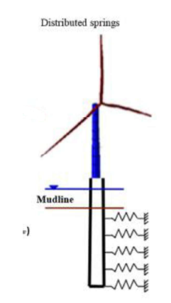
Figure 1 : Distributed springs along a pile with mudline
Soil-structure interactions are complex, and simplified approaches have been developed in the Oil & Gas industry to account for the coupling between the following typical structures:
- Jacket legs and the foundation
- The different casings of a drilling riser
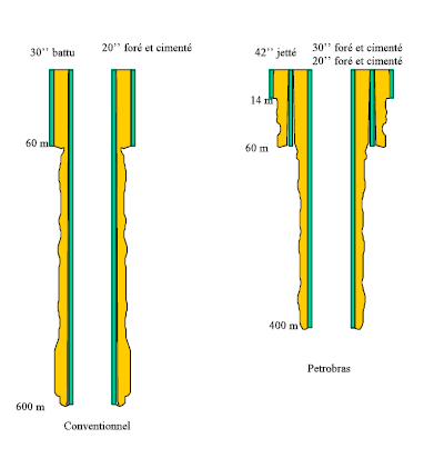
Figure 2 : Distributed springs along a pile with mudline
This relationship is commonly specified using semi-empirical functions based on experimental tests.
2.1. Context
- P–y: Lateral force vs. lateral displacement
- T–z: Longitudinal friction vs. vertical displacement along the pile (friction)
-
Q–z: Bearing force at pile tip vs. vertical displacement
Note
No other boundary conditions are considered (free to rotate).
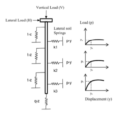
Figure 3 :
Classical P/y curves give the reaction force versus lateral displacement, while T/z curves often represent a friction law.
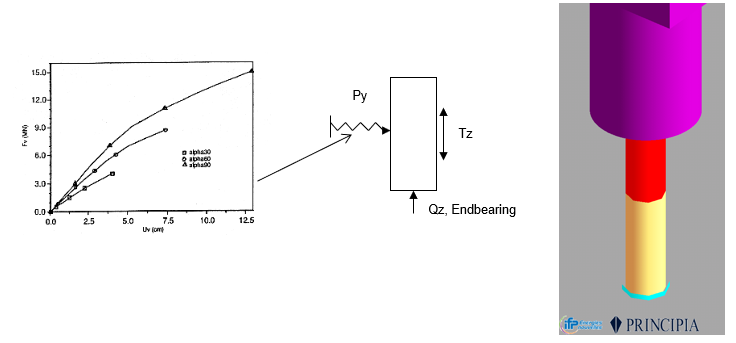
Figure 4 :
2.2. P–y / T–z Curves
Standard piles in the Oil & Gas industry are studied based on p–y / t–z curves according to API RP 2A §6 Foundation Design, which is dedicated to steel cylindrical pile foundations.
- Equations are valid for long piles with small diameter
- Not adapted for large monopiles and short cylinders
- Equations proposed for soft clays and sand
P–y curves are the most important to model because they:
- Impact the natural modes of the structure
-
Impact the stress distribution all along the structure
-
T–z and Q–z curves impact only the piles
- When piles are designed to be supported vertically in the soil (by friction and end bearing), the only impact is the stress distribution along the embedded part of the pile
- No impact on the structure above the mudline
Concept Stage Practice
- P–y curves are modeled with only one vertical support (at tip)
- Vertical reaction is checked and pile capacity is calculated to define:
- Required pile length
- Spudcan requirement (not performed in DLW)
- T–z & Q–z curves are added during detailed phases
- Adding these curves early can lead to model instability if pile capacity is not checked
- T–z is less relevant when spudcans are used
Spudcan Modeling Recommendations
For spudcan, ISO 19905-1 Part 1: Jack-up §9.3.4 provides additional recommendations for spudcan modeling.
Formulations exist (cf A.9.3.4.1) to provide:
- Vertical stiffness
- Horizontal stiffness
- Rotational stiffness
These are to be applied at the spudcan location.
2.3. Calculation method in DLW
2.3.1. The physics
The foundation is defined by the interface in the form:
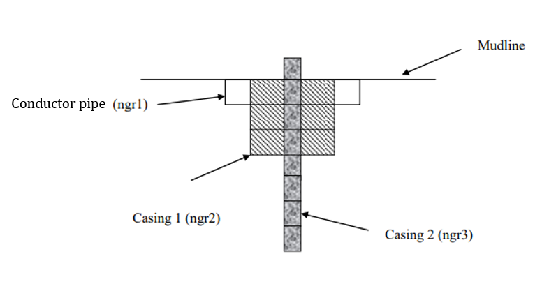
Figure 6 : Interface definition
We consider here the case of two casings. On each section, the nodes defining the inner tubes are slaves to the node at the same elevation that belongs to the outermost tube (cemented case).
Another possibility is to make the extreme nodes slaves if the tubes are not cemented, but in that case, a sliding contact type between the tubes must be defined.
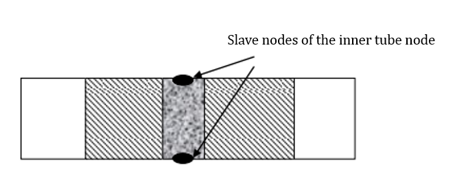
Figure 6 : Vizualisation of the slave nodes
The user or the interface has therefore defined at least two groups (or more if there are several casings), with master-slave relationships between the nodes of the outer tube and those of the inner tubes depending on the depth, or sliding-type relationships in the case where the inner tube is only fixed at the ends.
2.3.2. In DLW
For each foundation, the z-position of the last element of the foundation risers is calculated. This information is stored in fonpro(nfond, zn).
To add the forces, we go through the elements of a group, having verified that it is part of a foundation. For each Gauss point, the elevation is determined. Using the fonpro table, we deduce the outermost tube of the foundation at that level. If the node does not belong to this tube, no additional force is considered. Otherwise, it is subjected to a force from the soil. This force is provided by calculation procedures that determine the Py-Tz curves given by APIs or entered by the user. If the tube is located above the mudline, no force is applied.
In static analysis, the forces apply to an element in contact with the soil:
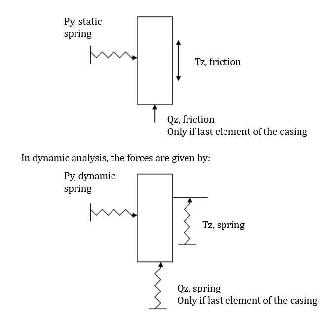
*Figure 4 : *
For Deeplines computation, an estimation of the derivative of the force is necessary for the numerical scheme. Forces of type Py, Tz, or Qz depend on the displacement vector relative to an initial position.
They can be expressed in the general form:
where \( \vec{u} \) is the displacement vector and \( P' \) is the force amplitude as a function of displacement.
The coordinates of the vector \( \vec{u} \) in a fixed reference frame are \( u_i, i=1,3 \). The derivative of the force with respect to a vector \( e_j \) with coordinates \( e_{i,j}, i=1,3 \) is a 3×3 matrix with components:
The forces depend on the position \( \bar{x}_t \) and the normal to the structure \( \bar{n} \).
For the Py force, the displacement is given by:
where \( x_s \) is the initial position vector.
The most important derivative is with respect to position. Since only an estimate of the derivative is needed (not its exact value), only the derivative with respect to position is provided here:
and thus:
The displacement along z is given by:
$$ u_t = (x_t − x_s )_s n_t n $$ The derivative with respect to position is then:
2.3.3. Input File Creation
- Mudline definition:
*DEPTH - Soil layers definition:
*GROUNDDEPTH - Soil type definition:
*GROUNDPROP - Curve definitions:
*PYCURVEand*TZCURVE - Foundation definition:
*FONDATION
The foundation refers to groups previously defined by *CASING for the casings. The type of installation is also specified.
Pipe/casing connections are also provided via *SLAVE and *TYPCONTACT.
2.3.4. Outputs
The outputs to be added are soil effort curves of the type displacement/reaction maximums with respect to depth.
Two specific soil databases are defined in static (.dss) and dynamic (.dst).
A first series of questions in Podeep proposes results in static (g) and dynamic (h) for the soil if the corresponding databases are available.
The results presented are forces and displacements, axial and lateral, of the outermost tube at a given depth.
For the static option, the questions are:
Step evolution <t>, Snapshot <f>, Other analysis <o>, exit<q>
Then:
Type of results:
Lateral displacement.............<l>
Lateral force....................<f>
Axial displacement...............<a>
Axial force......................<r>
Other............................<o>
Exit.............................<q>
If only one static step is defined, option <t> brings back the same menu.
Otherwise, two depths below the mudline must be entered, as well as the number of calculation points between these depths.
If the entered option is <f>, the number of the quasi-static step is requested after the depths.
For option <t>, the number of calculation points is limited to 10.
For the dynamic option, the questions are:
Step evolution <t>, Snapshot <f>, Envelop <e>, Other analysis <o>, exit<q>
Then:
Type of results:
Lateral displacement.............<1>
Lateral force....................<2>
Axial displacement...............<3>
Axial force......................<4>
Other............................<5>
Exit.............................<q>
The option <t> requires the minimum and maximum depths as well as the number of divisions (less than or equal to 10).
The option <x> requires the minimum and maximum depths as well as the number of divisions, then proposes either times chosen by the program over a period (where nn is the number of times, less than or equal to 10) or user-chosen times (enter b, then on the next line specify the times, fewer than 10).
The option <e> requires the minimum and maximum depths as well as the number of divisions.