Home > User Interface > Results Processing > Fatigue Analysis > Fatigue Analysis Setup > Specific option: mooring chain link fatigue analysis (OPB/IPB)

Specific option: mooring chain link fatigue analysis (OPB/IPB)

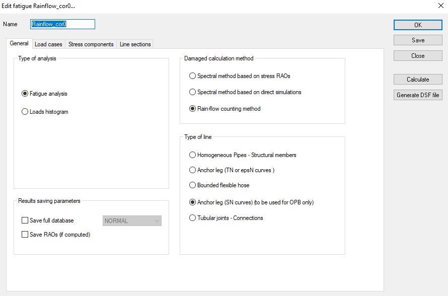
This option is selected through the option "Anchor leg (SN curves) (to be used for OPB only)". A specific line is usally defined with each element length equal to the interlink lengh (where contact occurs between links) and specific flexjoints elements between those beam elements to represent the interlink stifness (linear or non linear).

A post-treatment of the stress is done at 4 points as shown in the picture below. This cannot be changed by the user unless only axial stress are selected. In that case only one section point is computed.

The formula to generate the stress is based on the IPB and OPB moment in the link and is defined by (for axial plus bending) as:

For bending or axial+bending stresses, the stresses are computed with + or - M OPB combined with + or - M IPB resulting in four combinations (and physically corresponding to 4 points on the link). The SCFs are therefore combined SCFs: they are extracted at the same location on the link. Note the factor 2 on the axial stress reconstitution. The element should be a beam type of elements ("flexible type"). The diameter used is the outside diameter defined in "stress post-processing only" section of the flexible properties. The corrosion thickness defined in the same panel is also used unless a specific "corrosion thickness allowance" is selected in the "Stress components" of the fatigue analysis (see above panel). Note that with a corrosion thickness t , the diameter is reduced by t.

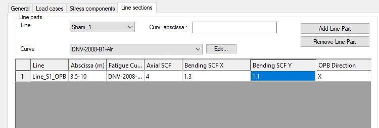
In the Line section, the line to be post-treated is defined together with the abscissa and SN curves. The three SCFs are defined. The bending SCFs are defined with respect to the local bending axis of the link (X and Y). Yhe OPB direction of your link must be defined to properly defined how to apply Z OPB and Z IPB.

Note that in the summary files of the fatigue analysis the bending SCFs written are different from the OPB and IPB SCFs entered in the interface. There is a factor \(\sqrt2\) on the OPB SCF and \(\sqrt2 \frac{Z_{OPB}}{Z_{IPB}}\) on the IPB SCF. This is due to the use of the OPB stress as a reference bending stress in OPB/IPB analyis (stress defined by \(\frac{M_{OPB}}{Z_{OPB}}\)), together with the formula defined below with \(SCF_{A_{C}}=SCF_{A_{S}}=SCF_{T-T}\). \(\sqrt2\) compensates the \(\frac{\sqrt{2}}{2}\) in the formula in bending directions.

\(\small\sigma_{G2}(t)=\frac{1}{2}(SCF_{A_{C}}+SCF_{A_{S}})\cdot\sigma_{AZ}(t)+\frac{\sqrt{2}}{2}\cdot SCF_{M_{IP}}\cdot\sigma_{FY}(t)-\frac{\sqrt{2}}{2}\cdot SCF_{M_{OP}}\cdot\sigma_{FX}(t)\)

\(\small\sigma_{G4}(t)=\frac{1}{2}(SCF_{A_{C}}+SCF_{A_{S}})\cdot\sigma_{AZ}(t)-\frac{\sqrt{2}}{2}\cdot SCF_{M_{IP}}\cdot\sigma_{FY}(t)-\frac{\sqrt{2}}{2}\cdot SCF_{M_{OP}}\cdot\sigma_{FX}(t)\)

\(\small\sigma_{G6}(t)=\frac{1}{2}(SCF_{A_{C}}+SCF_{A_{S}})\cdot\sigma_{AZ}(t)-\frac{\sqrt{2}}{2}\cdot SCF_{M_{IP}}\cdot\sigma_{FY}(t)+\frac{\sqrt{2}}{2}\cdot SCF_{M_{OP}}\cdot\sigma_{FX}(t)\)

\(\small\sigma_{G8}(t)=\frac{1}{2}(SCF_{A_{C}}+SCF_{A_{S}})\cdot\sigma_{AZ}(t)+\frac{\sqrt{2}}{2}\cdot SCF_{M_{IP}}\cdot\sigma_{FY}(t)+\frac{\sqrt{2}}{2}\cdot SCF_{M_{OP}}\cdot\sigma_{FX}(t)\)

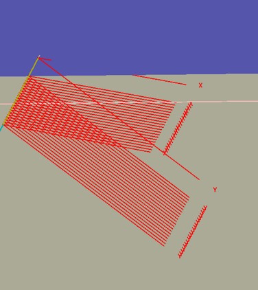
The local axis depends on the setting of your model. You can check the local direction after a static analysis by requiring the local axis of your mooring line (modelled as beam element at least for the section where OPB/IPB fatigue is required):