Home > User Interface > Results Processing > Fatigue Analysis > Fatigue Analysis Setup > Tubular joints - Connections (by subjoint)
Tubular joints - Connections (by subjoint)
Prerequisites
Fatigue analysis applied to this type of tubular intersection assumes that subjoints have been defined beforehand.
The various steps involved in defining these subjoints are summarized below.
Joint definition
A joint is a set of connected tubes which are not necessarily in the same plane.
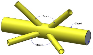
A joint has main aligned members called chords whose diameter are greater than the other connected tubes which are called braces :
The Tubular joints section explains how to define joints in DeepLines.
The following screenshot of the Edit Group of joints... dialog box shows for example the definition of the joint named Joint_28:
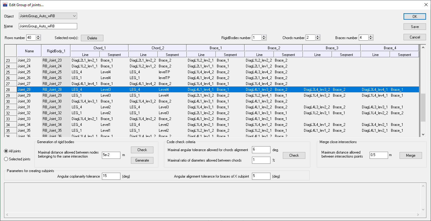
This joint has a chord line composed of 2 tubes (LEG_4/Level3, LEG_4/Level4) and 4 braces (DiagL4L1_lev4_1/Brace_1, DiagL4L1_lev3_2/Brace_2, DiagL3L4_lev3_2/Brace_2, DiagL3L4_lev4_1/Brace_1). Note that a tube is identified by the mention of the line and a segment.
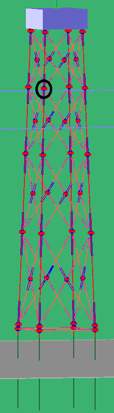
This joint belongs to a jacket and it is circled in black in the figure below:
Subjoint definition
A subjoint is a set of connected tubes belonging to a joint which are in the same plane. The fatigue computation is done on subjoints.
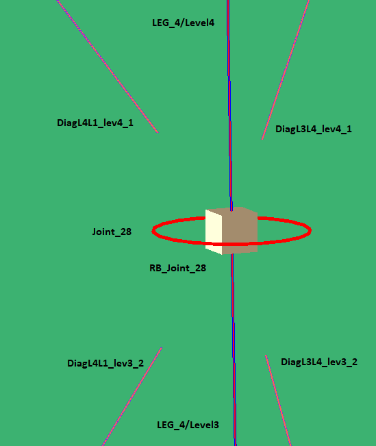
In the figure above, the joint has two subjoints because the braces are divided according to two planes:
-
one with the two braces DiagL4L1_lev3_2/Brace_2 and DiagL4L1_lev4_1/Brace_1,
-
the other with the two braces DiagL3L4_lev3_2/Brace_2 and DiagL3L4_lev4_1/Brace_1
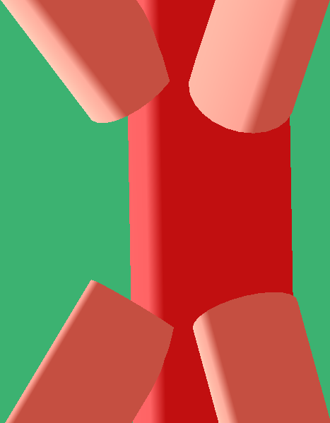
as can be seen in the filled view below:
With DeepLines, subjoints can be created automatically from the defined joints as explained in the Tubular joints : stiffnesses and Stress Concentration Factors section.
The following screenshot of the Edit Subjoints properties object... dialog box shows for example the definition of the subjoints obtained from the joint Joint_28:
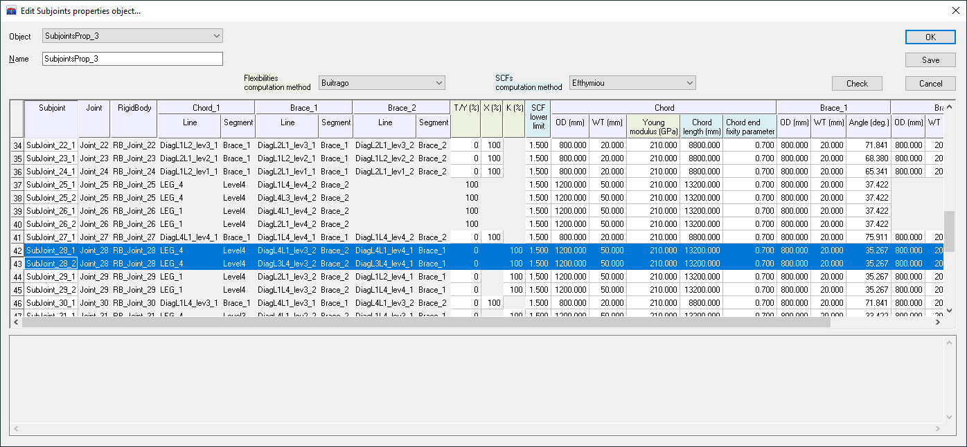
The table of subjoints definition and properties is filled with the default properties of the tubes (including geometric properties such as diameter, thickness, and the angle between the brace and the chord line) and can be changed by the user (for cells in background color white). Properties only used for the stiffnesses computation (with the Buitrago method) have their column titles in green and those used only for SCF calculations (with the Efthymiou method) have their column titles in blue.
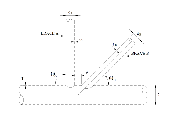
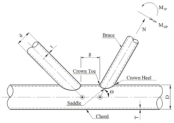
The figure below indicates these geometrical properties in the case of a K-subjoint:
Stiffnesses computation
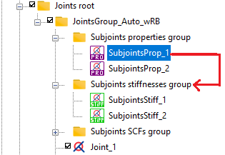
To define stiffnesses on subjoints, simply drag the Subjoints properties object into the Subjoints stiffnesses group folder:
The Edit Subjoints stiffnesses object dialog box opens with the computed stiffnesses for each brace of subjoint:
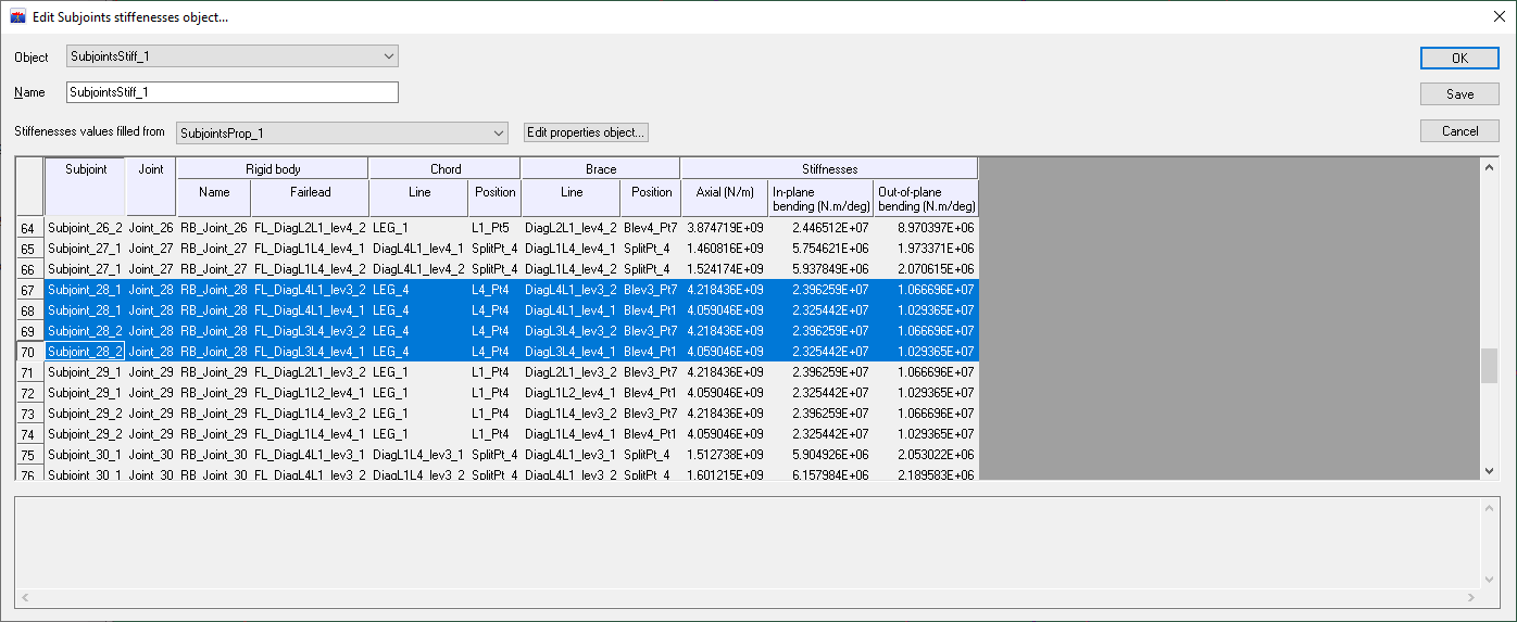
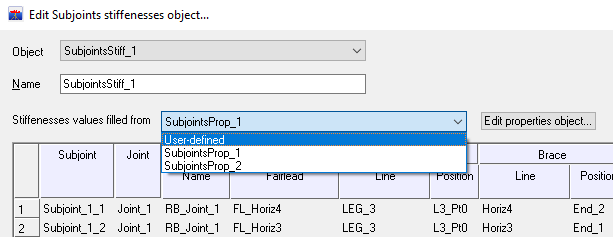
The name of the Subjoints properties object containing the tubes properties from which the stiffnesses were computed is shown above the table. If the user wants to enter his own values, he must select the User-defined item in the drop-down list and the default values can be overwritten:
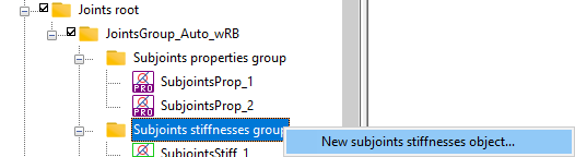
Alternatively, a new Subjoints stiffnesses object can be created by selecting the item of the contextual menu of the Subjoints stiffnesses group:
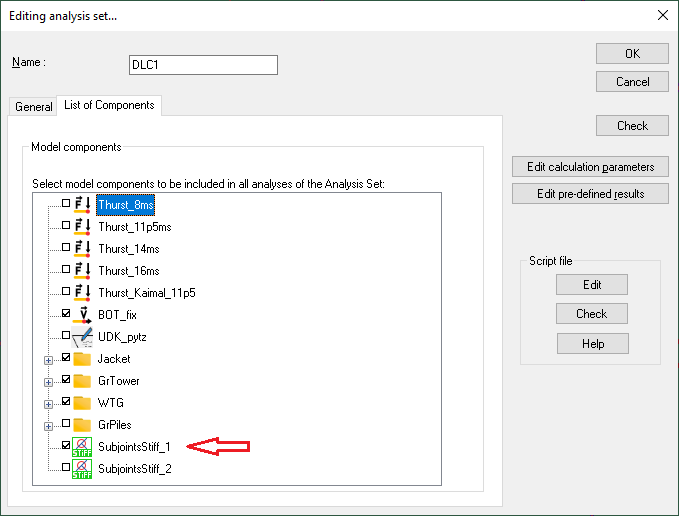
To take into account the subjoints stiffnesses in an analysis performed by the solver, select the Subjoints stifnesses object in the list of the analysis components:
For the Buitagro's parametric expressions for flexibilities see for example DNVGL-ST-0126, APPENDIX A LOCAL JOINT FLEXIBILITIES FOR TUBULAR JOINTS, April 2016.
Stress Concentration Factors computation
For fatigue calculations, it is necessary to create a Subjoints SCFs object using a method similar to that of a Subjoints stiffnesses object: simply drag the Subjoints properties object into the Subjoints SCFs group folder and a dialog box opens with the SCF computed with the Efthymiou method:
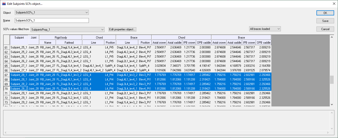
For each brace, they are 8 Stress Concentration Factors, 4 for the chord side and 4 for the brace side (Axial crown, Axial saddle, IPB crown, OPB saddle):
As for the stiffnesses, by selecting the User-defined item in the SCFs values filled from drop-down list, the user can overwrite the default values by his own values.
For the Efthymiou's expressions for SCF see for example DNV-RP-C203, APPENDIX B STRESS CONCENTRATION FACTORS FOR TUBULAR JOINTS, September 2021.
Definition of a fatigue analysis on subjoints
To define a fatigue analysis on subjoints, select the appropriate Type of line in the General tab of the Edit fatigue dialog box:
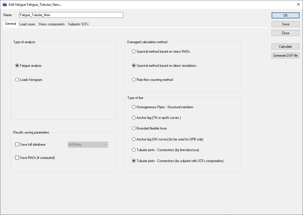
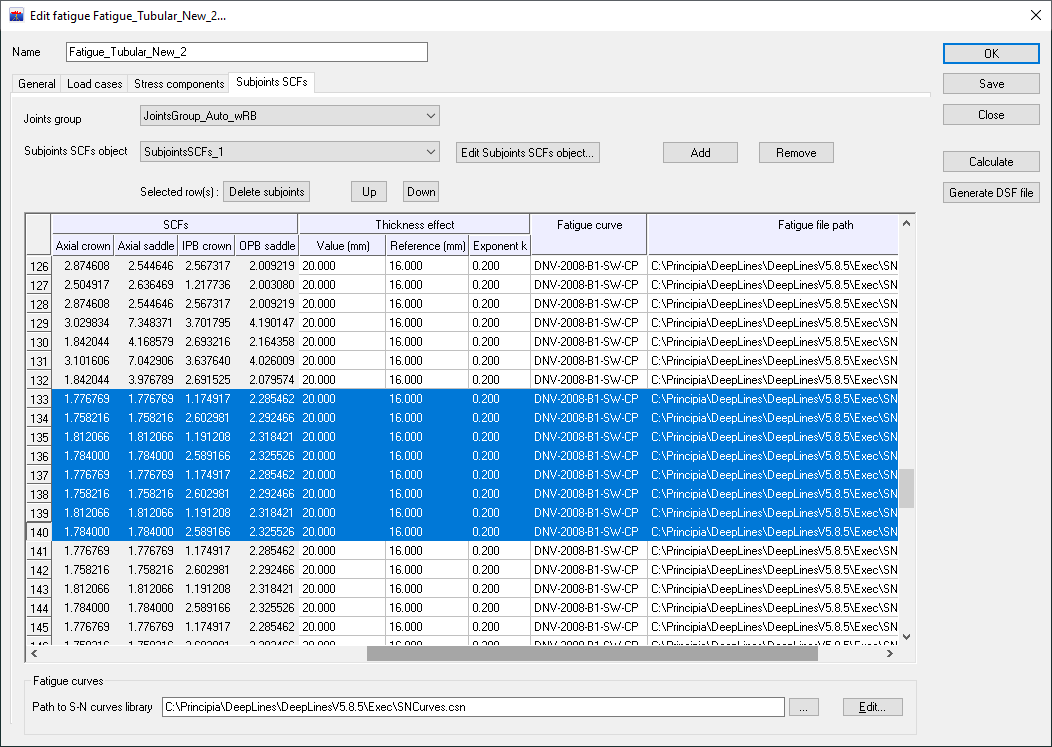
A Subjoints SCFs tab appears in the dialog box, and select a Subjoints SCFs object in the drop-down list:
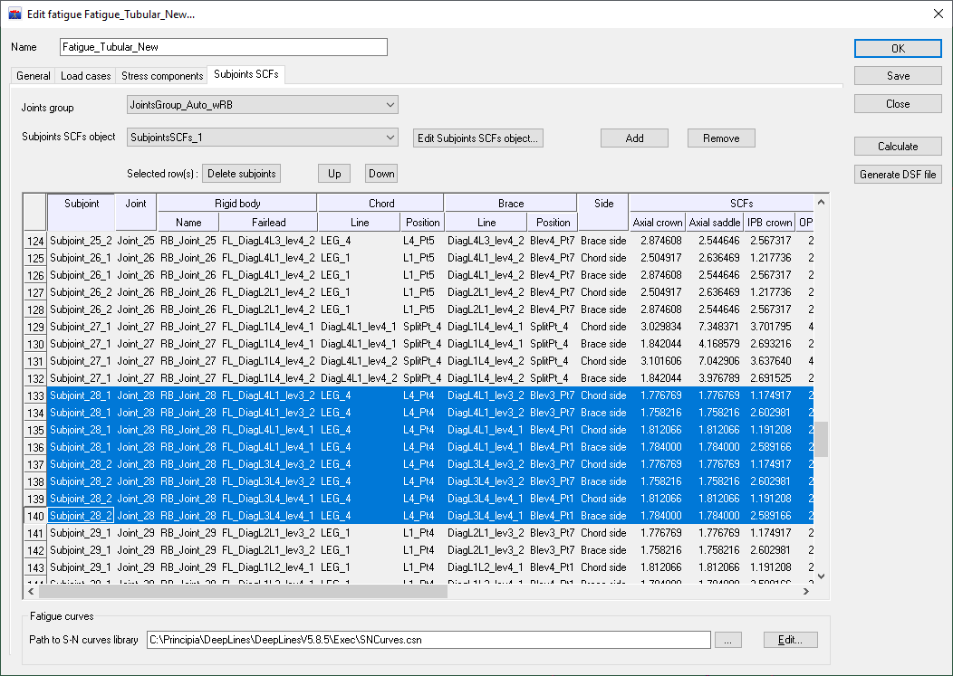
The table displays subjoints and their SCF contained in the Subjoints SCFs object. Note that the SCF for each brace are distributed on two lines: one for the chord side, the other for the brace side. The last columns allows the user to choose the fatigue curve.
If not all joints should be included in the analysis, it is possible to remove them by selecting the rows in the table and then pressing the Delete subjoints button.
The Add button allows the user to add Subjoints SCFs objects coming from other joints group.
Launching a fatigue analysis on subjoints
To launch interactively the fatigue analysis, press the Calculate button. Once the calculation is complete, two results folders are created: their names begin with the fatigue analysis name following by the _ChordSize and _BraceSide suffixes. The output files created in these folders depend of the type of Damaged calculation method chosen in the General tab, but a summary file is always created in text and Excel format which gives for each subjoint the maximal damage over the load cases. These must be defined in the Load cases tab.
To launch a fatigue analysis in batch refer to Running the Fatigue Analysis section.
Formulation
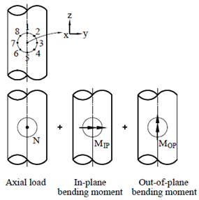
For each intersection, 8 stresses are calculated at 8 spots around the circumference of the intersection on the brace side and the same number on the chord side with the appropriate SCF :
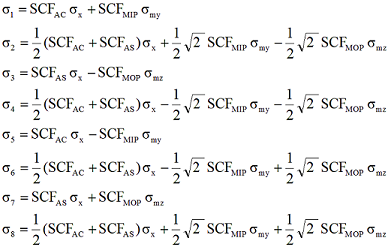
Here \(\mathsf{σ_x}\), \(\mathsf{σ_{my}}\) and \(\mathsf{σ_{mz}}\) are the maximum nominal stresses due to axial load and bending in-plane and out-of-plane respectively. \(\mathsf{SCF_{AS}}\) is the stress concentration factor at the saddle for axial load and the \(\mathsf{SCF_{AC}}\) is the stress concentration factor at the crown. \(\mathsf{SCF_{MIP}}\) is the stress concentration factor for in plane moment and \(\mathsf{SCF_{MOP}}\) is the stress concentration factor for out of plane moment.
Optional effects
The Stress components tab allows to take into account in the fatigue calculation two optional effects:
Thickness effect
The thickness effect is mentioned in the API-RP-2A-WSD 21st edition Rev 3 October 2007, § 5.5.2 Thickness effect:
where:
-
\(t_{ref}=\) the reference thickness (16 mm by default)
-
\(S=\) allowable stress range
-
\(S_0=\) allowable stress range from S-N curve
-
\(t\) member thickness for which the fatigue life is predicted
-
\(k\) exponent (0.2 by default)
No effect shall be applied to material thickness less than the reference thickness.
Once the thickness effect is selected, three new columns grouped under the heading Thickness effect appear which allow the user to specify the \(t\), \(t_{ref}\) and \(k\) parameters:
Chord effect
The chord effect is described in the API-RP-2A-WSD 21st edition Rev 3 October 2007, § C5.3.1.a Evaluation of Hot Spot Stress Ranges: the axial+bending stress of the chord is added to the efforts of the 6 spots around the circumference of the intersection which concern the chord crown.